Simple 3-Group Example

Model Description

The model divides reef organisms into three broad functional groups based on diet: predators, herbivores, and a general group of benthic invertebrates. This simple trait-based model is a smaller, three-group counterpart to the 10-group Karpata Reef model, useful when a coarser resolution is sufficient or as a starting point for setting up a new reef model. Both models are parameterised from the same marine-reserve dataset (see below); the 10-group model splits these same three broad functional groups (predators, herbivores, invertebrates) into finer functional groups. Estimates of observed biomass for each group were used to tune reproduction and resource consumption parameters so that steady state abundances agree with empirical observations. The process of establishing a steady state that agrees with empirical observations is nontrivial. Steady state parameters were tuned following the procedure described on the mizer blog. The R script used to tune the steady state parameters is included at the end of this file.

Biomass estimates were based on data collected from relatively un-fished reefs within a marine reserve in Bonaire. This data was part of the FORCE dataset that categorised fish community structure and habitat complexity across Caribbean coral reefs (Rogers et al. 2014, Williams et al. 2015, 2016, Newman et al. 2015, Dryden 2016). A marine-reserve site was chosen deliberately, for this model and for the 10-group Karpata Reef model alike, so that observed biomasses would not need to be corrected for fishing pressure before being used to calibrate the models. Visual surveys recorded fish up to 5 cm in length. The cutoff weight for observed biomass estimates was calculated using published length-weight relationships (Froese and Pauly 2023). The cutoff size is given in the table below along with the observed biomass per square meter in grams.

Species Group	Observed Biomass [g/m^2]	Cutoff Size [g]
predators	107	3.125
herbivores	34	3.125
inverts	40	3.125

Size Spectrum Dynamics

Skip to Resources

These dynamics expand on those used in standard Mizer models, see Delius et al. (2023).

Growth

The growth of organisms is dependent on the energy they are able to obtain from consumed food resources.

Predator-prey encounter rate

The rate $E_{i}(w)$ at which a predator of species $i$ and weight $w$ encounters food is dictated by the predation power $\gamma_i(w)$ , interaction matrix $\theta_{ij}$ , the vulnerability to predation $V_{ij}(w_p)$ , and the size selectivity of predator, given by the predation kernel $\phi_i(w,w_p)$ .

Interaction Matrix

The $\theta_{ij}$ matrix sets the interaction strength between predator group $i$ prey group $j$ . The predator/prey interaction matrix has entries between 0 (if the groups can not interact) and 1, see the figure below.

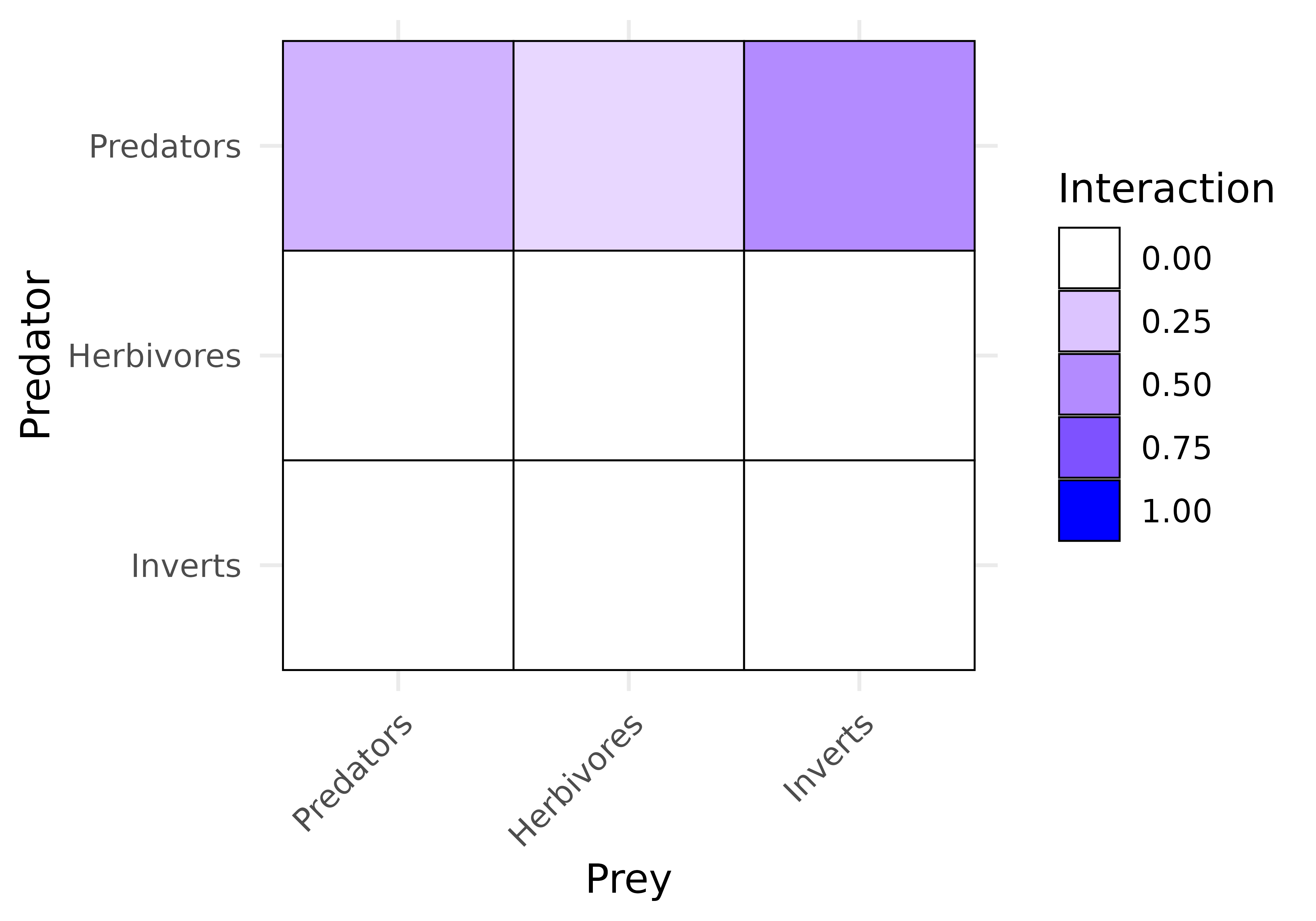
Interaction strength between each predator group (rows) and prey group (columns). Predators consume all three groups, at different strengths; herbivores and invertebrates do not prey on fish.

Predation Kernel

The parameters for the predation kernels were based on the global average predator prey mass ratio for marine organisms and home range size estimates from Nash et al. (2014). All estimates fall within observed ranges. All groups use a lognormal predation kernel with the same parameters as in Rogers et al. (2014). The parameters are given in the table below.

	beta	sigma	gamma
predators	100	1	0.4951721
herbivores	100	1	1.1517509
inverts	100	1	2.2473433

Vulnerability to Predation

The refuge function, $R_j(w_p)$ , describes the proportion of fish of size $w_p$ in prey group $j$ that are hidden from predators. $1 - R_j(w_p)$ is then the proportion of fish of weight $w_p$ and prey group $j$ that are vulnerable to consumption by predators. This model uses the method to determine the refuge profile, the set of proportions that describe refuge availability across the entire size range of model fish (Rogers et al. (2018)). The proportion of prey of weight $w_p$ and group $j$ with access to refuge $R_j(w_p)$ is given by

$R_j(w_p) = min\left \{R_{max} \, , \frac{\tau\cdot\eta_k}{\sum_{i}\int_{w_{k-1}}^{w_k} N_i(w)~dw} ~~~~~~~ w_p \in (~w_{k-1}, w_k~] \right \}$ {#eq-refuge_data}

The parameter $\tau$ is the proportion of fish with access to refuge that are expected to utilize it, $\eta_k$ is the density ( $no./m^{2}$ ) of refuges in size range $(w_{k-1}, w_k]$ and $\sum_{i} \int_{w_{k-1}}^{w_k} N_i(w)~dw$ gives the total density ( $no./m^{2}$ ) of fish from any group in size range $(w_{k-1}, w_k]$ . This represents the density of competitors for refuges in size class $k$ . With this method, the refuge profile is density dependent.

All fish are assumed to utilize refuge ( $\tau = 1$ ). Fish smaller than 0.1 g are assumed to be larval reef fish that have not yet settled to the reef. A maximum proportion of 98 % of fish are protected at any given time.

Refuge length bins and densities used in the steady state (same Bonaire FORCE data as the 10-group model)

The following table gives the fish length bins and refuge densities that define the refuge profile used in the steady state. Length bins and refuge densities were garnered from the FORCE data in the same location as biomass estimates - the same karpata_refuge profile used by the 10-group model.

Start of Bin (cm)	End of Bin (cm)	Refuge Density (no./m^2)
0	5	7.533
5	10	1.400
10	15	0.708
15	20	0.283
20	25	0.100
25	30	0.050
30	35	0.042
35	40	0.033
40	45	0.033
45	50	0.042

How each species group interacts with predation refuge

Each species group can utilise benthic structures differently depending on their specific traits. The table below indicates how each species group interacts with structures that provide predation refuge.

Group	Uses refuge?	Accesses prey in refuge?
predators	Yes	×
herbivores	Yes	Yes
inverts	×	Yes

The figure below shows the density-dependent refuge profile produced by the competitive method for the simple trait-based Caribbean 3-group model at steady state. Invertebrates are not shown as they do not use refuge (refuge_user = FALSE, see the table above).

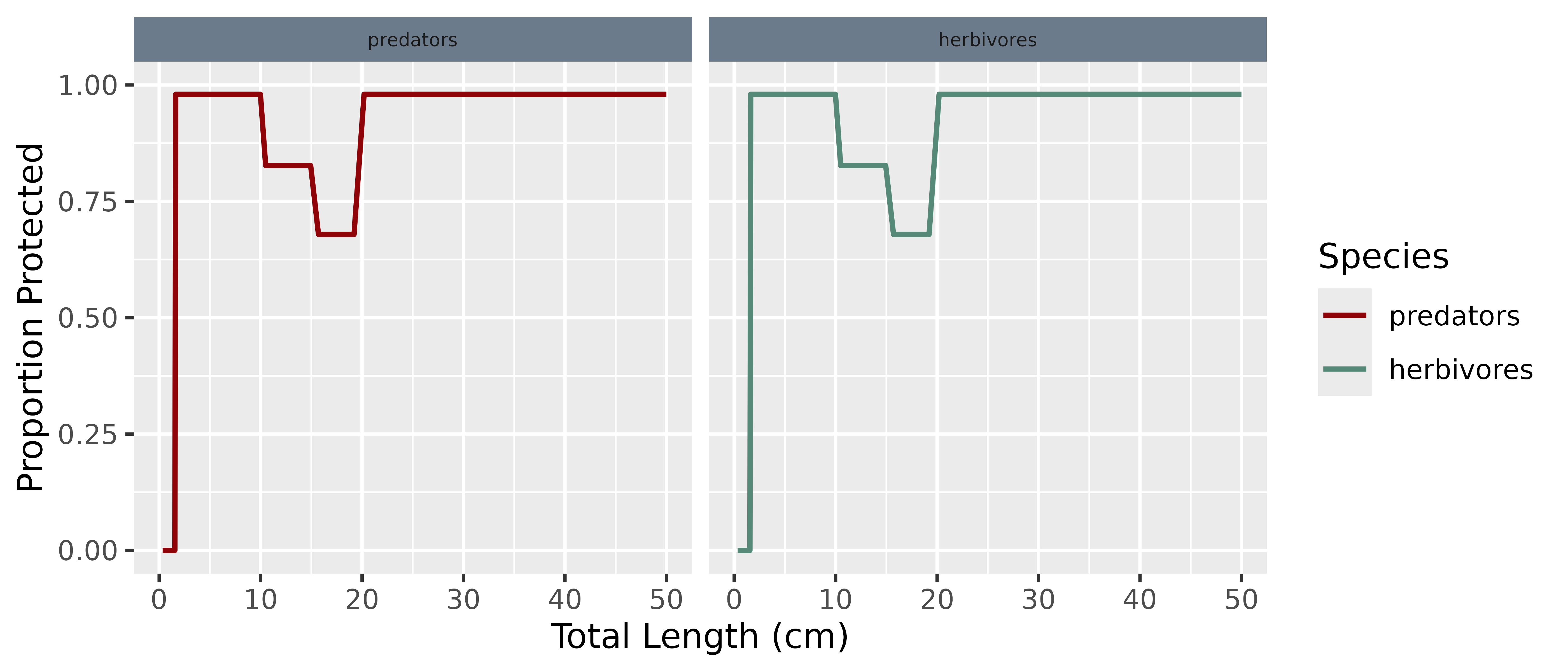
Proportion of each refuge-using group protected from predation, by body length, at steady state.

Consumption

Consumption of the detrital and algal resources is subject to a Holling functional response type II to represent satiation. This relationship is defined by the maximum intake rate, which increases allometrically with body size at rate $n$ . The parameter $h$ is the max consumption rate for a consumer of size 1 gram. Values for $h$ were chosen so that consumers subject to satiation are neither too starved nor totally satiated.

Only a proportion $\alpha_i$ of consumed biomass is retained, while a proportion $1-\alpha_i$ is expelled in the form of feces, which contribute to the detritus. See the table below for the max consumption rate for species subject to satiation.

No maximum consumption rate is imposed for predators. Herbivores are subject to satiation here, unlike the package default for herbivorous groups (see the main model description): recalibrating this model against the corrected senescence-mortality formula showed herbivore biomass has no density-dependent brake at all without some cap on individual intake once mortality is realistically low. The realised feeding level for herbivores is consistently close to 1, consistent with Caribbean herbivores’ guts being observed to be full essentially continuously (Ferreira et al. 1998, Kopp et al. 2010) – the citations behind the package’s herbivore-satiation default describe grazing pressure on the shared algae resource not self-regulating when food is abundant, which is unaffected by this change (see the main model description’s Algae section).

	h	alpha	n
herbivores	15.37483	0.6	0.75
inverts	30.00000	0.6	0.75

Metabolic Losses

The energy losses to metabolic needs are comprised of two components. Standard metabolism occurs at rate $k_{s.i}$ , scaling allometrically with body size at rate $p$ . The units of the coefficients $k_{s.i}$ are $\text{grams}^{1-p}$ per year. Losses due to activity and movement occur at rate $k_i$ in grams per year, scaling with body size at rate $1$ .

	ks	p
predators	0.0797345	0.75
herbivores	0.1236395	0.75
inverts	0.1000000	0.75

Energy Invested into Reproduction

A proportion $\psi_i(w)$ of the energy available for growth and reproduction is used for reproduction. This proportion changes from zero below the weight $w_{mat.i}$ of maturation to one at the maximum weight $w_{max.i}$ , where all available energy is used for reproduction.

Maturation length and age data were based on the most commonly observed species from each functional group in the FORCE data set (Rogers et al. 2014, Williams et al. 2015, 2016, Newman et al. 2015, Dryden 2016). For predators, this was the graysby grouper, Cephalopholis cruentata. The most commonly observed herbivore was the stoplight parrotfish, Sparisoma viride. Relevant maturity parameters were pulled from FishBase (Froese and Pauly 2023).

The herbivore age_mat value is set to 1.6 years, the age at median sexual maturity (AM50) reported for S. viride by Hernández and Shervette (2025) – a 2013-2023 otolith/gonad-histology study of 1801 U.S. Caribbean stoplight parrotfish. An earlier version of this model used age_mat = 4, which appears to have conflated AM50 with that same study’s age at median sexual transition (AT50 = 4.5 years, the age at which female stoplight parrotfish – a protogynous hermaphrodite species – become male), a distinct milestone from first reproductive maturity.

	w_mat	w_max	age_mat
predators	100.0	3125	4.0
herbivores	100.0	3125	1.6
inverts	0.1	3125	NA

Somatic growth

What is left over after metabolism and reproduction is taken into account is invested in somatic growth. Thus the growth rate of an individual of functional group $i$ and weight $w$ is $g_i(w) = E_{r.i}(w)\left(1-\psi_i(w)\right).$ {#eq-growth} When food supply does not cover the requirements of metabolism and activity, growth and reproduction stops, i.e. there is no negative growth. There is no starvation mortality in mizerReef.

The values for the model parameters were chosen so that the resulting growth curves would be close to von Bertalanffy growth curves. The parameters in the table below were taken from the literature.

	k_vb	w_max	a	b
predators	0.4	3125	0.025	3
herbivores	0.6	3125	0.025	3
inverts	NA	3125	0.025	3

Here the parameters $a$ and $b$ are parameters for the allometric weight-length relationship $w = a l^b$ where $w$ is measured in grams and $l$ is measured in centimetres.

Mortality

The mortality rate $\mu_i(w)$ of an individual of group $i$ and weight $w$ has three sources: predation mortality $\mu_{p.i}(w)$ , external mortality $\mu_{ext.i}(w)$ , fishing mortality $\mu_{f.i}(w)$ . External mortality is composed of residual natural mortality $\mu_{nat.i}(w)$ , and senescence $\mu_{sen.i}(w)$ . The mortality rate for group $i$ is then given by: $\mu_i(w)=\mu_{p.i}(w)+\mu_{ext.i}(w)+\mu_{f.i}(w)$ {#eq-mort}

Predation mortality

All consumption by fish translates into corresponding predation mortalities on the ingested prey individuals. the rate at which all predators from $j$ consume prey of size $w_p$ is $\mathtt{pred\_rate}_j(w_p) = \int \phi_j(w,w_p) \gamma_j(w) N_j(w) \, dw.$ {#eq-pred_rate}

The mortality rate due to predation is then obtained as $\mu_{p.i}(w_p) = \sum_j \mathtt{pred\_rate}_j(w_p)\, V_{ji}(w_p)\, \theta_{ji}.$ {#eq-mup}

Fishing Mortality

Like in mizer, fishing mortality in mizerReef is imposed by fishing gears. The total per-capita fishing mortality (1/year) is obtained by summing over the mortality from all gears,

$\mu_{f.i}(w) = \sum_g F_{g,i}(w)$

where the fishing mortality $F_{g,i}(w)$ imposed by gear $g$ on group $i$ at size $w$ is calculated as:

$F_{g,i}(w) = S_{g,i}(w) Q_{g,i} E_{g}$

The constant $S$ is the selectivity by group, gear and size, $Q$ is the catchability by group and gear and $E$ is the fishing effort by gear.

Fishing parameters for mizerReef models can be set up with setFishing(), which contains the details of how to set up gears with different selectivities and catchabilities for each group.

Fishing mortality $\mu_{f.i}(w)$ is calculated with the function getFMort(). The vignettes were run with following fishing parameters (the table below).

Group	Minimum fishing size [g]	Catchability [1/year]
predators	100	1
herbivores	100	1

External Mortality

Residual natural mortality

Mortality caused by illness, fishing, or predators not explicitly included in the model is captured by $\mu_{nat.i}(w)$ , which is independent of the functional groups and group abundances. It is assumed to decrease allometrically with body size:

$\mu_{nat.i}(w) = \mu_{nat} w^{1 - n}$ {#eq-z0} where $\mu_{nat}$ is the residual natural mortality rate and $n$ is the allometric scaling exponent. We use a residual mortality rate of $\mu_{nat} =$ 0.2 per year at size 1 gram.

Senescence mortality

Senescence mortality $\mu_{sen.i}(w)$ is intended to capture mortality due to illness or old age. It is independent of group abundances. Senescence mortality is assumed to increase allometrically with body size. The rate of senescence mortality is given by:

$\mu_{sen.i}(w) = k_{sen} \left(\frac{log_{10}(w)} {log_{10}(w_{max.i})}\right)^{p_{sen}}$ {#eq-extmort} with the ratio floored at zero for $w < 1$ g. Here $k_{sen}$ (sen_prop) is the rate the curve approaches as $w \to w_{max.i}$ , and $p_{sen}$ (sen_curve) controls the steepness with which mortality climbs as individuals approach their maximum size, and $w_{max.i}$ is the maximum body size of functional group $i$ in grams.

Senescence mortality due to illness and old age uses $k_{sen} =$ 0.1 and $p_{sen} =$ 0.3 for this model.

Reproduction

The reproduction parameters $\epsilon_i$ and $R_{max.i}$ are not directly observable. The values were instead chosen so as to produce steady-state abundances of the groups that are in line with observations and to give reasonable values for the reproduction level.

The table below gives the steady-state reproduction level $e\_repro$ which is defined as the ratio between the actual reproduction rate $R_i$ and the maximal possible reproduction rate $R_{\max.i}$ .

	w_min	erepro	R_max
predators	0.001	0.0012751	3.6103618
herbivores	0.001	0.0000180	0.3182451
inverts	0.001	0.0000598	9.0677690

Resources

Skip to Tuning the Steady State

The fish spectrum is fed by three background resources: plankton, algae, and detritus. Small individuals of all species will feed on plankton while only herbivorous groups and invertebrates feed on algae or detritus. The general mathematical form of the algae and detritus dynamics – a linear production/consumption balance for each pool, solved analytically each time step – was adapted from Delius et al. (2022, de Juan et al. 2023). This is not a direct port: mizerShelf represents its detritus/carrion pools by rescaling the total biomass of mizer’s size-structured background resource spectrum, whereas mizerReef’s algae and detritus are genuinely unstructured scalar pools with their own dedicated encounter-rate matrices, added as independent components via setComponent(). mizerReef also adds coral-reef-specific behaviour with no equivalent in mizerShelf, most notably that algae production is treated as a fixed rate of primary production decoupled from consumer demand rather than tuned to match consumption (see algae_consumption()’s documentation for the ecological rationale and citations).

Plankton

The plankton spectrum $N_P(w)$ tracks the abundance all planktonic food sources. This spectrum starts at a smaller size than the fish spectrum in order to provide food for the smallest individuals (larvae) of the fish spectrum.

The plankton spectrum ranges from $w_0=9\times 10^{-13}$ to $w_{cutoff}=1$ grams. The steady state abundance of plankton at size 1 gram is $\kappa=5.87 (g/m^{2})$ . The slope of the plankton spectrum is set to $\lambda=2.05$ .

Algae

The algal resource is described only by its total biomass $B_A$ . Feeding on algae is not size-based. Herbivores can feed on algae of any size. In the steady state the total algal biomass per square meter is $B_A = 2.17\times 10^{-10}$ grams.

Algal consumption

For each consumer species $i$ , a parameter $\rho_{A.i}$ determines the rate at which individuals of that species encounter algal biomass. The parameters $\rho_{i.A}$ have units of $g^{-n}$ per year. They are non-zero only for species that consume at least some algae. The preference $\theta_{i.A}$ for algae is a value between 0 and 1 specifying the proportion of consumer diets that are comprised of algal matter.

	rho	interaction_algae
herbivores	611046350815	1

Algal production

The rate at which algal biomass is produced by the ecosystem is given by a constant growth rate with units of grams per unit area per unit time. At steady state algal production is 2000 grams per square meter per year.

Detritus

Detritus is consumed by herbivores and benthic invertebrates. Feeding on detritus is not size-based as fish can feed on detritus particles of any size. The detritus resource is described only by its total biomass $B_D$ . In the steady state the total detrital biomass per square meter is $B_D = 5.871\times 10^{-11}$ grams.

Detrital consumption

For each consumer species $i$ , a parameter $\rho_{D.i}$ determines the rate at which individuals of that species encounter detritus. The parameters $\rho_{i.D}$ have units of $g^{-n}$ per year. They are non-zero only for species that consume at least some detritus. The preference $\theta_{i.D}$ for detritus is a value between 0 and 1 specifying the proportion of consumer diets comprised of detritus.

	rho	interaction_detritus
inverts	1.192299e+12	1

Detrital production

Detritus comes from defecation and decomposing dead organisms that die as a result of sources of external mortality. At steady state detritus from decomposing dead organisms is 119.45 g/year and defecation produces 176.05 g/year. A proportion ext_decomp of the external mortality and a proportion sen_decomp of senescence mortality decomposes to detritus. The proportion of detritus that sinks from external mortality is 80 % and the proportion that decomposes from senescence mortality is 80 %. These values are based on estimates from Hatcher (1988).

External detritus is generated by unmodelled sources or sinks in from the pelagic zone. At steady state external detritus production is -110.76 g/year. This value is set so that steady state abundances match empirical observations. Where it is negative, feces and mortality are producing more detritus than can be consumed. Detrital biomass is assumed to be washed away by wave action in this case.

Tuning the Steady State

The following R script was used to tune the steady state parameters for this model (see inst/scripts/Caribbean_3_model-calibration.R in the package source for the exact, currently-runnable version).

Show the full steady-state calibration script

# Setting up a generic Caribbean coral reef model with multiple resources
# Three groups: Predators, Herbivores, Invertebrates
# Model steady state calibration

## Setup - load packages --------------------------------------------------
library(mizer)
library(mizerExperimental)
library(mizerReef)
library(here)

## Load parameters ----------------------------------------------------------
caribbean_3_species <- read.csv(here("inst/data-csv/caribbean_3_species.csv"))
caribbean_3_interaction <- read.csv(here("inst/data-csv/caribbean_3_interaction.csv"),
                                    row.names = 1)
# Refuge densities from Karpata reef in Bonaire, FORCE dataset
karpata_refuge <- read.csv(here("inst/data-csv/karpata_refuge.csv"))
tuning_profile <- read.csv(here("inst/data-csv/tuning_profile.csv"))

# With these parameters, herbivores consume plankton at small sizes and
#   transition fully to algae by maturity
# With these parameters, invertebrates consume plankton and detritus,
#   with the proportion of detritus increasing with size

## Set model -----------------------------------------------------------------
params <- newReefParams(
    species_params = caribbean_3_species,
    interaction = caribbean_3_interaction,
    method = "binned",
    method_params = tuning_profile
)

## Project to first steady state ----------------------------------------------
params <- reefSteady(params)

## Calibrate biomasses and growth ----------------------------------------------

# Match observed species group biomasses
params <- calibrateReefBiomass(params)
params <- matchBiomasses(params)
params <- reefSteady(params)

# Match observed growth rates
params <- matchReefGrowth(params)
params <- reefSteady(params)

# Iterate to refine biomass - repeat many times; piping keeps it readable.
params <- params |>
    calibrateReefBiomass() |> matchBiomasses() |> matchReefGrowth() |>
    reefSteady() |>
    calibrateReefBiomass() |> matchBiomasses() |> matchReefGrowth() |>
    reefSteady() |>
    calibrateReefBiomass() |> matchBiomasses() |> matchReefGrowth() |>
    reefSteady()
# (repeated several more times in the full calibration script until
#  plotBiomassVsSpecies(params) matches observations closely)

plotBiomassVsSpecies(params) # spot on
plotTotalAbundance(params)
plotTotalBiomass(params)

## Now switch to competitive method ---------------------------------------------
params <- newRefuge(params,
    new_method = "competitive",
    new_method_params = karpata_refuge
)

# Match biomasses again with the new refuge profile
params <- params |>
    calibrateReefBiomass() |> matchBiomasses() |> matchReefGrowth() |>
    reefSteady() |>
    calibrateReefBiomass() |> matchBiomasses() |> matchReefGrowth() |>
    reefSteady()
# (repeated several more times in the full calibration script)

# Make sure new refuge is in place
plotVulnerable(params)
plotRefugeProfile(params)
plotBiomassVsSpecies(params) # spot on

## Check resulting spectra and tune resources ------------------------------------

# Spectra should be reasonably straight to match predictions of Sheldon's
# spectrum but also have nonlinearities at refuge sizes
plotSpectra(params, total = TRUE, power = 1)
plotSpectra(params, total = TRUE, power = 2)
plotFeedingLevel(params, species = "inverts")

# Tune reproduction -----------------------------------------------------------
# We do not have yield or catch data - can't tune size distribution
params <- setBevertonHolt(params, erepro = 0.0134)
params <- reefSteady(params)

# Increase reproduction level to reduce excessive density dependence
rep_level <- c(0.5, 0.5, getReproductionLevel(params)["inverts"])
names(rep_level) <- c("predators", "herbivores", "inverts")
params <- setBevertonHolt(params, reproduction_level = rep_level)

# Iterate to get back to steady state
params <- params |> reefSteady() |> reefSteady() |> reefSteady()

# Final diagnostic plots
plotBiomassVsSpecies(params)
plotRefugeProfile(params)
plotSpectra(params, power = 1, total = TRUE)
plotDiet(params)
plotGrowthCurves(params)
plotPredMort(params)

# Save!
caribbean_3_model <- reefSteady(params)
save(caribbean_3_model, file = "data/caribbean_3_model.rda")

de Juan, S., G. Delius, and F. Maynou. 2023. A model of size-spectrum dynamics to estimate the effects of improving fisheries selectivity and reducing discards in mediterranean mixed demersal fisheries. Fisheries Research 266:106764.

Delius, G., S. de Juan, and F. Maynou. 2022. mizerShelf: Mizer models with carrion and detritus components suitable for continental shelf ecosystems.

Delius, G., F. Scott, J. Blanchard, and K. Andersen. 2023. Mizer: Dynamic multi-species size spectrum modelling.

Dryden, C. 2016. Habitat structural complexity of caribbean coral reefs and its relationships with fish community structure. PhD thesis, Newcastle University, Newcastle upon Tyne United Kingdom.

Ferreira, D. E. L., A. C. Peret, and R. Coutinho. 1998. Seasonal grazing rates and food processing by tropical herbivorous fishes. Journal of Fish Biology 53:222–235.

Froese, R., and D. Pauly. 2023. FishBase.

Hatcher, B. G. 1988. Coral reef primary productivity: A beggar’s banquet. Trends in Ecology & Evolution 3:106–111.

Hernández, J. M. R., and V. R. Shervette. 2025. Addressing life history information gaps for Caribbean parrotfishes: Queen parrotfish Scarus vetula and stoplight parrotfish Sparisoma viride. Environmental Biology of Fishes 108:179–198.

Kopp, D., Y. Bouchon-Navaro, S. Cordonnier, A. Haouisée, M. Louis, and C. Bouchon. 2010. Evaluation of algal regulation by herbivorous fishes on caribbean coral reefs. Helgoland Marine Research 64:181–190.

Nash, K. L., J. Q. Welsh, N. A. J. Graham, and D. R. Bellwood. 2014. Home-range allometry in coral reef fishes: Comparison to other vertebrates, methodological issues and management implications. Oecologia 177:73–83.

Newman, S. P., E. H. Meesters, C. S. Dryden, S. M. Williams, C. Sanchez, P. J. Mumby, and N. V. C. Polunin. 2015. Reef flattening effects on total richness and species responses in the caribbean. Journal of Animal Ecology 84:1678–1689.

Rogers, A., J. L. Blanchard, and P. J. Mumby. 2014. Vulnerability of coral reef fisheries to a loss of structural complexity. Current Biology 24:1000–1005.

Rogers, A., J. L. Blanchard, S. P. Newman, C. S. Dryden, and P. J. Mumby. 2018. High refuge availability on coral reefs increases the vulnerability of reef‐associated predators to overexploitation. Ecology 99:450–463.

Williams, S. M., I. Chollett, G. Roff, J. Cortaes, C. S. Dryden, and P. J. Mumby. 2015. Hierarchical spatial patterns in caribbean reef benthic assemblages. Journal of Biogeography 42:1327–1335.

Williams, S. M., C. S’anchez?God’ınez, S. P. Newman, and J. Cort’es. 2016. Ecological assessments of the coral reef communities in the eastern caribbean and the effects of herbivory in influencing coral juvenile density and algal cover. Marine Ecology 38.

Caribbean 3-Group Steady State Model Description