The mizerReef size-spectrum model

Overview

This page gives a mathematical description of the mizerReef model. mizerReef is an extension of mizer, and this page assumes that you are already familiar with the general mizer model. We use the same notation as in the mizer model description and concentrate on the places where mizerReef departs from or adds to core mizer. Everything not mentioned here (the size-spectrum dynamics, the shape of the predation kernel, the growth and reproduction machinery, the fishing model, and so on) is inherited unchanged from mizer.

mizerReef is designed for structurally complex habitats such as coral reefs. It adds four ingredients to the standard multispecies model:

1. Predation refuge. Structural complexity lets some prey hide from some predators. This is captured by a size- and species-dependent vulnerability $V_{ji}(w)$ that discounts both the food a predator encounters and the predation mortality it inflicts.
2. Unstructured resources. In addition to the size-structured resource spectrum $N_R(w)$ (plankton), mizerReef tracks two non-size-structured benthic pools: algae with biomass $B_A$ and detritus with biomass $B_D$.
3. Satiation control. Individual consumer groups can be exempted from the Holling type II satiation response, so that carnivores take all the food they encounter.
4. Senescence mortality. An extra size-dependent mortality term $\mu_{sen.i}(w)$ acting near a group’s maximum size, on top of the residual natural mortality.

Throughout, the index $i$ (or $j$) runs over the modelled functional groups rather than taxonomic species; in mizerReef the entries of $N_i(w)$ are usually size spectra of feeding guilds.

State variables

A mizerReef model carries the same consumer spectra $N_i(w)$ and resource spectrum $N_R(w)$ as mizer, together with two additional scalar state variables:

• $B_A$, the total biomass of algae (turf, macroalgae and the epilithic algal matrix), and
• $B_D$, the total biomass of detritus (decomposing organic matter, faeces and material sinking in from the pelagic zone).

Neither pool is size-structured, reflecting the fact that reef herbivores and detritivores feed on these resources largely independently of their own body size. Their dynamics are given in the section on unstructured resource dynamics. They are stored as other components of the model (n_other$algae and n_other$detritus) and evolve alongside the fish and plankton spectra.

Predation refuge and vulnerability

The central mechanism in mizerReef is that habitat structure shelters prey from predators. We describe this with the vulnerability $V_{ji}(w)$: the proportion of individuals of prey group $i$ at size $w$ that are not hidden inside refuge and are therefore available to be encountered and eaten by predator group $j$. It is a dimensionless number between $0$ and $1$, computed by reefVulnerable() and returned by getVulnerable().

Two group-level flags in the species parameter table decide who is affected:

• refuge_user marks the prey groups $i$ that seek shelter. Groups that never use refuge have $V_{ji}(w) = 1$ for all predators and sizes.
• blocked_pred marks the predator groups $j$ whose foraging is obstructed by structure. A predator with blocked_pred = FALSE (for example an eel that can follow prey into a crevice) is unaffected by refuge and always sees $V_{ji}(w) = 1$.

Writing $R_i(w)$ for the proportion of refuge-using prey group $i$ that are sheltered at size $w$ (the refuge profile, defined below), the vulnerability is $$V_{ji}(w) = \begin{cases} 1 - R_i(w) & \text{if group } i \text{ uses refuge and predator } j \text{ is blocked,}\\ 1 & \text{otherwise.} \end{cases}$$ Because the sheltering depends on the prey only, $V_{ji}(w)$ takes just two possible values for each prey group and size — the discounted value $1-R_i(w)$ for blocked predators and $1$ for predators that can reach into refuge.

The refuge profile is capped at a maximum protection level, $R_i(w) \le r_{\max}$ (max_protect, default $0.98$), so that some food always remains accessible.

Refuge profiles

The refuge profile $R_i(w)$ is set with setRefuge(), which offers three ways to specify it plus a trivial “no refuge” option. All three convert between length and weight using length–weight parameters $a$ and $b$ (so that $w = a\, L^{b}$), using either group-specific values or a set of “dummy fish” values $\bar a, \bar b$, depending on how the field data were collected.

Sigmoidal. A smooth decline in protection around a threshold length $L_{\text{refuge}}$, appropriate when the refuge-size distribution is unknown. With threshold weight $W_{\text{refuge}} = a\,L_{\text{refuge}}^{\,b}$, $$R_i(w) = \frac{r}{1 + \exp\!\big(\Delta\,(w - W_{\text{refuge}})\big)},$$ where $r$ (prop_protect) is the maximum proportion protected and $\Delta$ (slope) sets the sharpness of the transition.

Binned. A step function that is appropriate for theoretical experiments. On a set of length bins with weight edges $w_{k-1} < w \le w_k$, $$R_i(w) = r_k \qquad \text{for } w \in (w_{k-1}, w_k],$$ with a constant protected proportion $r_k$ in each bin.

Competitive. The mechanistic, density-dependent option, used when the density of physical refuges is known. Let $\eta_k$ be the density of refuges (number per m²) in size bin $k$. These refuges are shared out among all refuge-using individuals whose size falls in that bin, so the protected proportion is the ratio of available refuges to competitors: $$R_i(w) = \min\!\left(r_{\max},\; \tau \, \frac{\eta_k} {\displaystyle\sum_{\ell}\int_{w_{k-1}}^{w_k} N_\ell(w')\,dw'}\right), \qquad w \in (w_{k-1}, w_k],$$ where the sum runs over all refuge-using groups $\ell$ and $\tau$ (tau, default $1$) is the fraction of individuals with access to a refuge that actually use it. When there are no competitors the protection is set to $r_{\max}$.

The competitive profile is the only one that couples back to the fish abundances: as a size class becomes crowded, the same number of refuges protect a smaller fraction of it, so vulnerability rises with density. This provides an additional, habitat-mediated source of density dependence that is recomputed at every time step. The static sigmoidal and binned profiles, by contrast, are fixed once set.

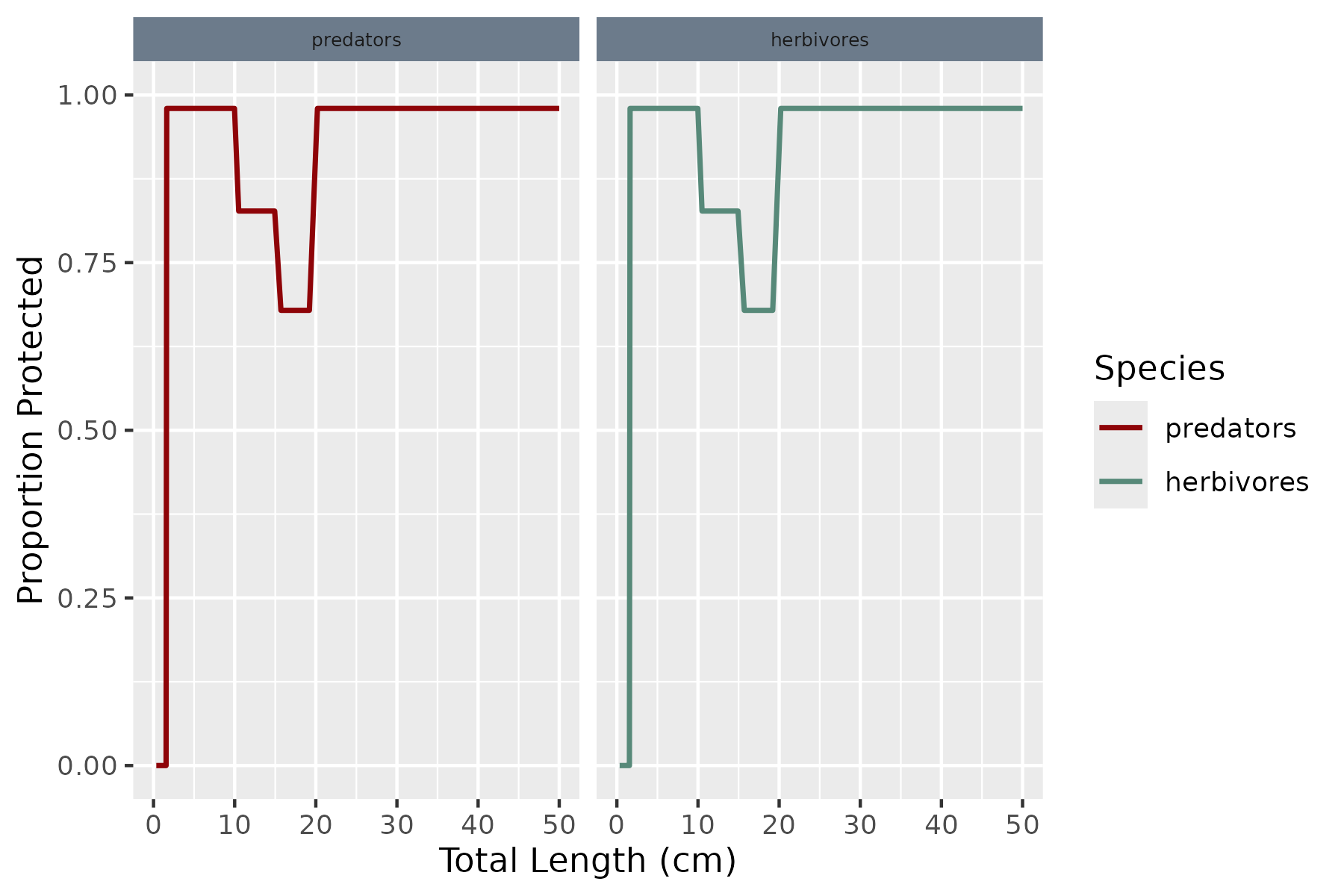
Refuge profile for the built-in Caribbean example model: the proportion protected by refuge as a function of body size for each functional group.

Habitat degradation

The competitive method also supports time-dependent loss of structure, used to simulate bleaching or physical damage (setDegradation(), reefDegrade()). The refuge density is scaled forward in time by a sequence of factors: from a bleaching time $t_{\text{bleach}}$ onwards, $$\eta_k(t) = s_k(t)\,\eta_k(t-1),$$ where the $s_k(t)$ are user-supplied scaling factors (the columns of deg_scale) giving the fractional change in refuge density in each successive year post-disturbance. Optionally the algal growth rate and carrying capacity can be boosted over the same period to represent the algal proliferation that often follows coral loss.

Encounter rate

The predation encounter rate has the same form as in mizer but with two modifications: prey abundances are discounted by their vulnerability, and the unstructured resources contribute additional, non-size-structured food.

For a predator of group $i$ and weight $w$, $$E_i(w) = \gamma_i(w) \int \left( \theta_{iR}\,N_R(w_p) + \sum_{j} \theta_{ij}\, V_{ij}(w_p)\, N_j(w_p) \right) \phi_i(w, w_p)\, w_p \, dw_p \;+\; E_{i,A}(w) + E_{i,D}(w).$$ Compared with mizer, the fish-prey term now carries the factor $V_{ij}(w_p)$, which removes the sheltered fraction of each prey group from the food available to predator $i$. The plankton resource $N_R$ is not affected by refuge. The search volume $\gamma_i(w)$, interaction coefficients $\theta_{ij}$, $\theta_{iR}$ and predation kernel $\phi_i$ are exactly as in mizer, and the integral is evaluated by the same fast Fourier transform when the kernel depends only on the predator/prey size ratio. This rate is computed by reefEncounter().

The last two terms are the contributions from feeding on the unstructured resources. Because these pools are not size-structured, the encounter rate on each is simply proportional to its total biomass: $$E_{i,A}(w) = \rho_{i,A}\,\theta_{i,A}\, w^{m_{alg}}\, B_A, \qquad E_{i,D}(w) = \rho_{i,D}\,\theta_{i,D}\, w^{m_{det}}\, B_D,$$ where $\theta_{i,A}$ and $\theta_{i,D}$ (interaction_algae, interaction_detritus) set each group’s preference for algae and detritus, the coefficients $\rho_{i,A}, \rho_{i,D}$ set the overall consumption power, and the allometric exponents $m_{alg}, m_{det}$ control how intake scales with consumer size. This contribution is added through mizer’s standard component mechanism (encounter_contribution()).

Consumption and satiation

As in mizer, encountered food is consumed subject to a Holling type II functional response, giving the feeding level $$f_i(w) = \frac{E_i(w)}{E_i(w) + h_i(w)},$$ where $h_i(w)$ is the maximum intake rate. The proportion $1 - f_i(w)$ of encountered food is actually consumed, and the absorbed rate available for metabolism, growth and reproduction is $\alpha_i (1 - f_i(w)) E_i(w)$.

mizerReef adds a per-group satiation switch (satiation). Groups with satiation = FALSE have no upper limit on their intake, formally $h_i(w) = \infty$. For them the feeding level collapses to $$f_i(w) = 0,$$ so they consume everything they encounter and the absorbed rate is simply $\alpha_i E_i(w)$. This behaviour is implemented by reefFeedingLevel(), which sets the maximum intake to infinity for non-satiating groups and treats the resulting $0/0$ feeding level as zero.

By default, only species that consume detritus but not algae (i.e. pure detritivores/invertebrates) keep the type II response (satiation = TRUE); carnivores and herbivores both default to satiation = FALSE (see setRefuge()), since satiation-mediated consumption is intended to be exclusive to detritivory — see the Algae section below for the citations behind this default for herbivores specifically. This is a default, not a hard rule: caribbean_3_model and caribbean_10_model (karpata) both override it to satiation = TRUE for their herbivore/parrotfish groups, because recalibrating those models against the corrected senescence-mortality formula showed herbivore biomass has no density-dependent brake at all without some cap on individual intake once mortality is realistically low (see inst/scripts/Caribbean_3_model-calibration.R‘s design note for the full reasoning) — the underlying “herbivores don’t reduce grazing pressure on the shared algae pool” claim these citations support is unaffected by this, since algae_consumption() (the resource-depletion rate) deliberately ignores feeding level regardless of any species’ satiation setting.

Growth and reproduction

The partitioning of absorbed energy into metabolism, growth and reproduction is unchanged from mizer. After metabolic losses $\text{metab}_i(w)$, the rate available for growth and reproduction is $$E_{r.i}(w) = \max\!\big(0,\; \alpha_i (1 - f_i(w))\, E_i(w) - \text{metab}_i(w)\big),$$ a fraction $\psi_i(w)$ of which goes to reproduction and the remainder to somatic growth, $g_i(w) = E_{r.i}(w)\,(1 - \psi_i(w))$. Reproduction uses the same egg-production integral and the same emergent Beverton–Holt stock–recruitment relationship as mizer. See the mizer model description for details.

Mortality

The total mortality on a consumer of group $i$ and weight $w$ is $$\mu_i(w) = \mu_{p.i}(w) + \mu_{nat.i}(w) + \mu_{sen.i}(w) + F_i(w),$$ computed by reefMort(). Fishing mortality $F_i(w)$ is exactly as in mizer. The remaining three terms differ from core mizer as follows.

Predation mortality

All food eaten becomes predation mortality on the prey, but only the vulnerable, non-sheltered individuals can be eaten. The predation mortality on prey group $i$ at size $w_p$ is $$\mu_{p.i}(w_p) = \sum_j \text{pred\_rate}_j(w_p)\, V_{ji}(w_p)\, \theta_{ji},$$ where $\text{pred\_rate}_j$ is the same predation rate as in mizer (computed from predator $j$’s feeding). The extra factor $V_{ji}(w_p)$ discounts the contribution of each predator $j$ by the fraction of prey $i$ that is exposed to it: predators that are blocked by refuge (blocked_pred = TRUE) only prey on the $1 - R_i(w_p)$ fraction that is out in the open, while predators that can reach into refuge apply the full mortality. This is computed by reefPredMort().

Residual natural mortality

Mortality from sources not modelled explicitly (predators outside the model, disease, and so on) is taken to be allometric in size, $$\mu_{nat.i}(w) = \mu_{nat}\, w^{\,1-n},$$ with $\mu_{nat}$ the rate at $1$ g (nat_mort, default $0.2$) and $n$ the growth exponent. This is mizerReef’s external mortality $\mu_{ext.i}(w)$ and plays the same role as $z0_i$ in mizer.

Senescence mortality

To represent death from old age near a group’s maximum size, mizerReef adds a size-increasing senescence term (reefSenMort(), getSenMort()): $$\mu_{sen.i}(w) = k_{sen}\, \left(\frac{\log_{10} w}{\log_{10} w_{max.i}} \right)^{p_{sen}},$$ with the ratio floored at zero for $w < 1$ g. Here $w_{max.i}$ is the maximum weight of group $i$, $k_{sen}$ (sen_prop) is the rate the curve approaches as $w \to w_{max.i}$ (where the ratio is exactly 1), and $p_{sen}$ (sen_curve) controls the steepness with which mortality climbs as individuals approach their maximum size. Senescence mortality is included only when the model is set up to use it; both it and the residual natural mortality are configured through setExtMortParams().

Resource mortality

Predation mortality on the plankton resource $N_R(w)$ is computed exactly as in mizer. The predation losses on the unstructured pools $B_A$ and $B_D$ are accounted for through their consumption terms in the dynamics below rather than as a size-resolved mortality.

Unstructured resource dynamics

The algae and detritus pools each obey a linear balance between production and consumption. Because they are single scalars, their dynamics are ordinary differential equations that mizerReef solves analytically over each time step of length $dt$, which avoids the numerical instability of an explicit Euler step. The general mathematical form of these dynamics – a linear production/ consumption balance for each unstructured pool, solved analytically each time step – was adapted from the mizerShelf extension package (Delius et al. 2022, de Juan et al. 2023). This is not a direct port, though: mizerShelf represents its detritus/carrion pools by rescaling the total biomass of mizer’s size-structured background resource spectrum, whereas mizerReef’s algae and detritus are genuinely unstructured scalar pools with their own dedicated species- and size-dependent encounter-rate matrices ($\rho$), added as independent components via setComponent(). mizerReef also adds coral-reef-specific behaviour with no equivalent in mizerShelf, most notably that algae production is treated as a fixed rate of primary production decoupled from consumer demand rather than tuned to match consumption (see algae_consumption()’s documentation for the ecological rationale and citations).

Algae

The algal biomass follows $$\frac{dB_A}{dt} = P_A - c_A\, B_A,$$ where $P_A$ is the production rate. Unlike detritus, algal production on a reef is real primary production and is not driven by grazer demand, so $P_A$ is a fixed, literature-informed constant (getAlgaeProduction(), see setAlgaeParams()) rather than something tuned to match consumption; instead it is the algae biomass $B_A$ that is solved for at steady state (tuneUR()/tuneUR_cc()), so that, all else equal, a decrease in grazing pressure increases the standing algae biomass rather than reducing modelled production to compensate. $c_A$ is the mass-specific consumption rate (algae_consumption()). The latter is the total rate at which consumers graze the pool per unit of algal biomass, $$c_A = \sum_i \int \rho_{i,A}\,\theta_{i,A}\, w^{m_{alg}}\, N_i(w)\, dw,$$ so that the total grazing rate is $c_A B_A$. Note that, unlike detritus consumption below, this deliberately does not include a feeding-level factor: in mizerReef, satiation-mediated consumption is exclusive to detritivory. Increases in herbivorous fish density following coral bleaching events suggest that reef herbivores respond to increased food availability without regulating their consumption (Ledlie et al. 2007, Pratchett et al. 2008, Khalil et al. 2013, Elma et al. 2023), and Caribbean herbivores have been observed to fill their gut up to three times a day (Ferreira et al. 1998, Kopp et al. 2010). Algal consumption is therefore modelled as driven by continuous grazing pressure regardless of the satiation setting for the herbivore species involved – see algae_consumption()’s documentation for more detail. Over a step the equation integrates to $$B_A(t + dt) = B_A(t)\, e^{-c_A\, dt} + \frac{P_A}{c_A}\left(1 - e^{-c_A\, dt}\right).$$

Detritus

Detritus obeys the same form, $$\frac{dB_D}{dt} = P_D - c_D\, B_D, \qquad B_D(t + dt) = B_D(t)\, e^{-c_D\, dt} + \frac{P_D}{c_D}\left(1 - e^{-c_D\, dt}\right),$$ with mass-specific consumption $$c_D = \sum_i \int \rho_{i,D}\,\theta_{i,D}\, w^{m_{det}} \big(1 - f_i(w)\big)\, N_i(w)\, dw$$ (detritus_consumption()). Unlike algae, detritus is produced by several processes in the ecosystem, and its production rate is the sum of three contributions (getDetritusProduction()): $$P_D = p_{D,f} + p_{D,d} + p_{D,\text{ext}}.$$

• Faeces — the fraction of consumed biomass that is not assimilated: $$p_{D,f} = \sum_i (1 - \alpha_i) \int \big(1 - f_i(w)\big)\, E_i(w)\, N_i(w)\, dw.$$
• Decomposing carcasses — a fraction of the biomass lost to residual natural and senescence mortality: $$p_{D,d} = c_{ext}\sum_i \int \mu_{nat.i}(w)\, N_i(w)\, w\, dw + c_{sen}\sum_i \int \mu_{sen.i}(w)\, N_i(w)\, w\, dw,$$ where $c_{ext}$ (ext_decomp) and $c_{sen}$ (sen_decomp) are the proportions of each mortality source that decompose to detritus rather than being exported.
• External input $p_{D,\text{ext}}$ — a constant rate at which detritus enters from unmodelled sources such as sponges, coral mucus and pelagic sinking (external), set to close the steady-state budget.

Carrying-capacity variant

For scenarios in which the benthos saturates, both pools can instead be given logistic production (setURcapacity(), algae_dynamics_cc(), detritus_dynamics_cc()): $$\frac{dB}{dt} = P\left(1 - \frac{B}{K}\right) - c\, B,$$ with carrying capacity $K$. This too is solved analytically over each step, $$B(t + dt) = B(t)\, e^{-\frac{dt}{K}(P + K c)} + \frac{K P}{P + K c}\left(1 - e^{-\frac{dt}{K}(P + K c)}\right),$$ and reduces to the linear case as $K \to \infty$.

Summary of differences from mizer

Process	mizer	mizerReef
Prey availability	full abundance $N_j(w)$	discounted by vulnerability $V_{ij}(w)\,N_j(w)$
Encounter	plankton + fish	plankton + fish + algae + detritus
Satiation	all groups	optional; off for carnivores
External mortality	constant $z0_i$	$\mu_{nat}\,w^{1-n}$ plus senescence $\mu_{sen.i}(w)$
Extra resources	resource spectrum only	plus unstructured pools $B_A$, $B_D$

For how these equations are realised through mizer’s extension mechanism (S3 dispatch, NextMethod() chaining and registered components), see the extension mechanism vignette.

de Juan, S., G. Delius, and F. Maynou. 2023. A model of size-spectrum dynamics to estimate the effects of improving fisheries selectivity and reducing discards in mediterranean mixed demersal fisheries. Fisheries Research 266:106764.

Delius, G., S. de Juan, and F. Maynou. 2022. mizerShelf: Mizer models with carrion and detritus components suitable for continental shelf ecosystems.

Elma, E., M. Gullström, S. A. S. Yahya, J.-B. Jouffray, H. K. East, and M. Nyström. 2023. Post-bleaching alterations in coral reef communities. Marine Pollution Bulletin 186:114479.

Ferreira, D. E. L., A. C. Peret, and R. Coutinho. 1998. Seasonal grazing rates and food processing by tropical herbivorous fishes. Journal of Fish Biology 53:222–235.

Khalil, M. T., J. E. M. Cochran, and M. L. Berumen. 2013. The abundance of herbivorous fish on an inshore red sea reef following a mass coral bleaching event. Environmental Biology of Fishes 96:1065–1072.

Kopp, D., Y. Bouchon-Navaro, S. Cordonnier, A. Haouisée, M. Louis, and C. Bouchon. 2010. Evaluation of algal regulation by herbivorous fishes on caribbean coral reefs. Helgoland Marine Research 64:181–190.

Ledlie, M. H., N. A. J. Graham, J. C. Bythell, S. K. Wilson, S. Jennings, N. V. C. Polunin, and J. Hardcastle. 2007. Phase shifts and the role of herbivory in the resilience of coral reefs. Coral Reefs 26:641–653.

Pratchett, M., P. Munday, S. Wilson, N. Graham, J. Cinner, D. Bellwood, G. Jones, N. Polunin, and T. McClanahan. 2008. Effects of climate-induced coral bleaching on coral-reef fishes: Ecological and economic consequences. Oceanography and Marine Biology: An Annual Review 46:251–296.