Getting started with MizerReef • mizerReef

Overview

The mizerReef package enables multi-species dynamic size-spectrum modelling in R, with an explicit, mechanistic representation of habitat structural complexity. In this vignette, we walk through the basic steps needed to build and explore your first MizerReef model, including:

Installing MizerReef
Setting species parameters
Setting the refuge profile
Creating your first model
Tuning the steady state
Exploring results
Changing the refuge profile
Running a simulation

Model context: Habitat structure mediates system dynamics by providing predation refuge. The most effective refuges fit prey while excluding predators, so refuge use is primarily governed by body size. In systems with high structural complexity (for example, coral reefs), these patterns are reflected in the size structure of fish assemblages.

Because refuge protection is size-dependent, size-spectrum models provide a natural framework for exploring how benthic structure influences community dynamics. MizerReef modifies predator–prey encounter rates to represent the effects of habitat structure, allowing users to explicitly account for changes in refuge availability caused by habitat degradation or modification.

For a detailed description of the model formulation and supporting references, see Chapter 3 of Modelling Coral Reef Futures: Exploring the role of structural complexity in sustaining ecosystem services (PhD Thesis, VUW).

MizerReef builds on the mizer package

MizerReef is an extension of the mizer package and uses many of the same functions and parameters. If you are new to mizer, want a refresher on the general workflow, or would like more background on size-spectrum modelling, visit the mizer website. You may also find the mizer course helpful.

Installing MizerReef

Skip to Setting up species parameters

MizerReef is currently only available from GitHub. To install the latest version, use the devtools package:

install.packages("devtools")
devtools::install_github("cmbeese/mizerReef")

MizerReef depends on the mizer and mizerExperimental packages. If not already installed, R will prompt you to install them automatically. Without them, you will not be able to use all of the features in mizerReef.

After installation, load Mizer, mizerExperimental, and MizerReef in each new R session:

library(mizer)
library(mizerExperimental)
library(mizerReef)

💡 Tip: Be sure to load mizerReef last. Some of the functions in mizerReef override functions in mizer, so loading in this order ensures that correct versions are used.

Use a recent version of R and RStudio for best results. For troubleshooting or more details, see the MizerReef documentation or the GitHub repository.

Setting species parameters

Skip to mizerReef parameters

The species parameter table is the foundation of any mizer or mizerReef model. It describes the biological and ecological traits of each species in your system.

💡 Tip: Many users prefer to create this table in a spreadsheet program (like Excel or Google Sheets) and then import it into R as a data frame.

Species parameters required by base mizer

For a multi-species mizer model, only the following columns are strictly required in the species parameter data frame:

species: Name of the species or group
w_max or l_max: Maximum observed weight or length (if providing length, you must also provide length-weight conversion parameters a and b)

By default, mizerReef creates multispecies mizer models.

mizerReef is not compatible with trait-based or community models at this time. See multispecies mizer models to learn more about the differences between the three model types in mizer.

You can tune your model to a specific system using abundance data if you also provide:

biomass_observed: Observed abundance for each species.
biomass_cutoff: Minimum weight of organisms caught by survey methods (helps with tuning)

The choice in units for your data is arbitrary as long as you are consistent.

Abundance data can be given as numbers per area, numbers per volume or total numbers for the entire study area. See Units in Mizer for more information.

Since MizerReef’s vulnerability and refuge dynamics depend on size, it is good to include parameters related to growth and size rather than relying on defaults, including:

w_mat: Maturity weight (important for life history & growth)
beta & sigma: Lognormal predation kernel parameters (set for each species, can use other kernels)
Length-to-weight conversion parameters a and b

You should also provide the interaction matrix, which specifies predator-prey relationships between species.

Each value in the interaction matrix, ranging from 0 to 1, represents the strength of interaction between a predator (row) and its prey (column). These can represent spatial overlap, diet preferences, or other ecological factors influencing predation rates.

It is important that the order of rows and columns in the interaction matrix matches the order of species in the species parameter data frame within the params object. To view the example interaction matrix included with MizerReef, run:

data("caribbean_3_interaction")
caribbean_3_interaction

See Setting Parameters in Mizer for details on additional optional columns and their defaults.

Additional species parameters needed for mizerReef

Skip to Example species parameters

mizerReef extends mizer by modeling reef-specific dynamics. To utilise the predation vulnerability and unstructured resource dynamics in MizerReef, add these columns to your species parameter data frame:

Additional columns required for mizerReef species parameters.
Column	Type	Description
refuge_user	logical	TRUE if the group uses predation refuge (i.e., individuals hide inside habitat structure to avoid predators; typical for small-bodied or cryptic reef fish). FALSE for species that do not use refuge. FALSE by default
blocked_pred	logical	TRUE if the group is blocked from accessing prey in refuge (i.e., predators that cannot reach prey hiding in refuge). FALSE for species with behavioural or morphological adaptations (e.g., eels) that allow them to access prey in refuge. FALSE by default.
satiation	logical	TRUE if group is subject to satiation on unstructured resources (algae or detritus; default is TRUE for herbivores, FALSE for carnivores).
interaction_algae	numeric	Proportion of diet from algae (0–1). 0 by default.
interaction_detritus	numeric	Proportion of diet from detritus (0–1). 0 by default

By default, MizerReef will assign values to any missing parameters so that the corresponding feature is disabled, and issue a warning. See [setRefuge()], [setAlgaeParams()] and [setDetritusParams()] for additional details.

💡 Tip: When importing your species parameter table from a CSV, make sure that missing values are represented as NA or blank cells, not zeros.
You can load your species parameter data frame into R using standard functions like read.csv() or readxl::read_excel(), depending on your file format. Ensure that the column names in your data frame match those expected by MizerReef. Use na.strings = c(““,” “) in read.csv() to ensure blanks are read as NA rather than 0.

Example mizerReef species parameters

Skip to Setting the refuge profile

MizerReef includes example model parameters with the package. See the Model Description for more details on these example data.

The included species parameter data frame (caribbean_10_species) is based on fish assemblage data from a Caribbean reef site with relatively low fishing pressure. The full species parameter data frame for the Caribbean 10 example is shown below:

species	l_max	w_mat	age_mat	beta	sigma	biomass_cutoff	biomass_observed	a	b	interaction_detritus	interaction_algae	refuge_user	blocked_pred	satiation
pred_eng	45	50.0	2.0	60	2	12.62969	5.51	0.01100	3.06	0.0	0.0	TRUE	TRUE	FALSE
pred_grab	60	140.0	5.4	40	2	17.80530	27.60	0.01740	3.01	0.0	0.0	TRUE	TRUE	FALSE
eels	100	300.0	3.0	30	2	NA	10.00	0.00098	3.24	0.0	0.0	TRUE	FALSE	FALSE
pred_crypt	8	0.8	NA	10	1	1.00000	NA	0.01122	3.04	0.5	0.0	TRUE	FALSE	FALSE
pred_inv	45	50.0	0.5	50	2	26.58539	14.13	0.01200	3.10	0.0	0.0	TRUE	FALSE	FALSE
pred_plank	20	2.5	1.0	1000	3	13.49043	0.55	0.01259	3.03	0.0	0.0	TRUE	FALSE	TRUE
parrotfish	64	63.0	1.6	30	1	15.48385	30.56	0.01380	3.05	0.5	0.5	TRUE	FALSE	TRUE
farm_damsel	13	1.0	1.0	30	1	NA	0.40	0.02042	2.97	0.5	0.5	TRUE	FALSE	TRUE
herbs	39	105.0	2.0	30	1	75.75344	1.50	0.02570	2.95	0.5	0.5	TRUE	FALSE	TRUE
inverts	30	0.1	NA	30	2	3.12500	NA	0.02500	3.00	1.0	0.0	FALSE	FALSE	TRUE

💡 Tip: The Karpata species parameters also include optional columns like w_mat, age_mat, k_vb, and ks. Include as many parameters as you have data for to assist in the calibration process.

Setting the refuge profile

Skip to Creating your first model

The refuge profile defines how predation refuge availability varies with prey size (see Figure 1). This is a key feature of MizerReef that allows you to represent the effects of habitat structure on predator-prey interactions.

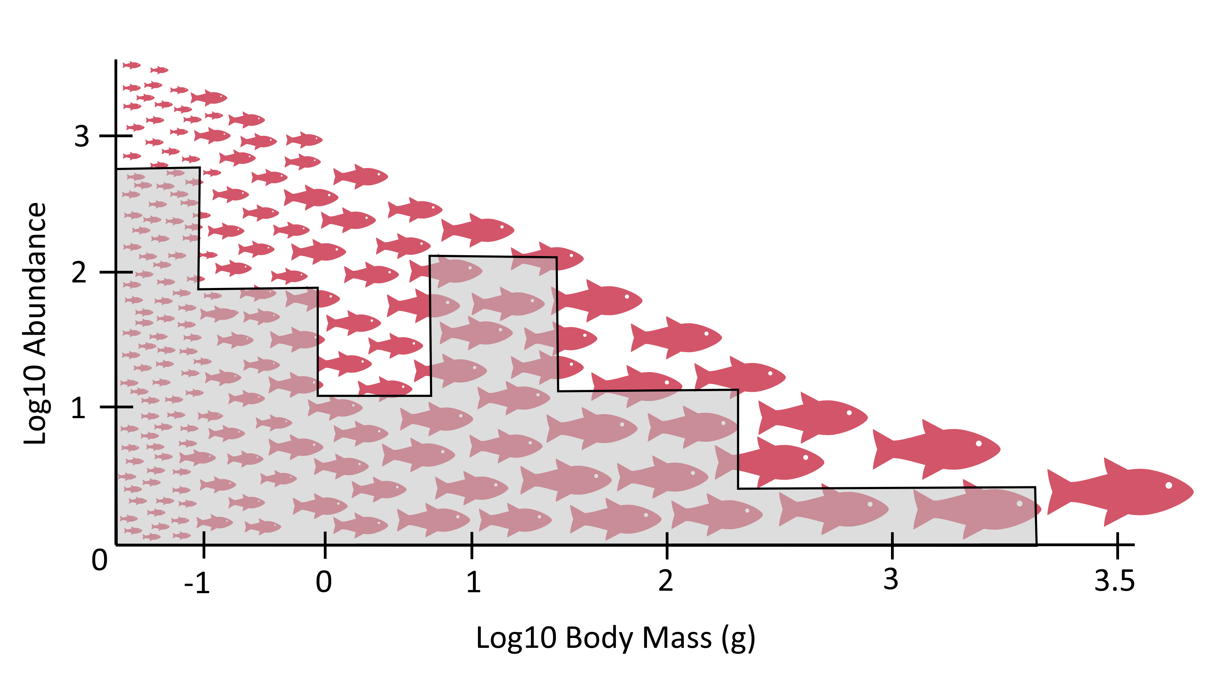
Figure 1. Conceptual schematic of the refuge profile. The red fish represents the modelled fish spectrum. Individuals protected from predators by refuge are covered by the grey box. The remaining individuals are vulnerable to predation.

MizerReef currently provides three methods to define how refuge availability varies with prey size:

Sigmoidal: Good for data-poor reefs or when you want a simple, smooth profile.

a smooth declining function controlled by a threshold length (L_refuge) and a maximum proportion protected
- method_params should be a list or data frame with:
  - L_refuge: numeric, threshold length (cm) at which refuge protection starts to decline.
  - prop_protect: numeric, maximum proportion of individuals protected by refuge (0–1).
Example:
```
method_params = list(L_refuge = 10, prop_protect = 0.8)
```

Binned: Good for theoretical experiments or when you have coarse bin information.

user-specified length bins with a constant protection proportion inside each bin
- method_params should be a data frame or matrix with two columns:
  - length_bin: numeric, the upper length (cm) of each bin.
  - protection: numeric, the proportion of individuals protected by refuge (0–1) within each length bin.
Example:
```
method_params = data.frame(
  length_bin = c(5, 10, 20, 40),
  protection = c(1, 0.5, 0, 0.2)
)
```

Competitive: divides refuges among similarly sized competitors. Use this when you have empirical refuge density data.

uses refuge density (no./m^2) for each length bin, protection depends on fish density within each bin (density-dependent)
- method_params should be a data frame or matrix with two columns:
  - length_bin: numeric, the upper length (cm) of each bin.
  - refuge_density: numeric, the density of refuges (no./m^2) available for each length bin.
Example:
```
method_params = data.frame(
  length_bin = c(5, 10, 20, 40),
  refuge_density = c(2, 1, 0.5, 3)
)
```

Refuge profiles and body shape

This plot shows example refuge profiles created using each method and how they differ based on species body shape characteristics. The same set of species groups can receive different protection based on their body shape, the chosen method, and method-specific parameters.

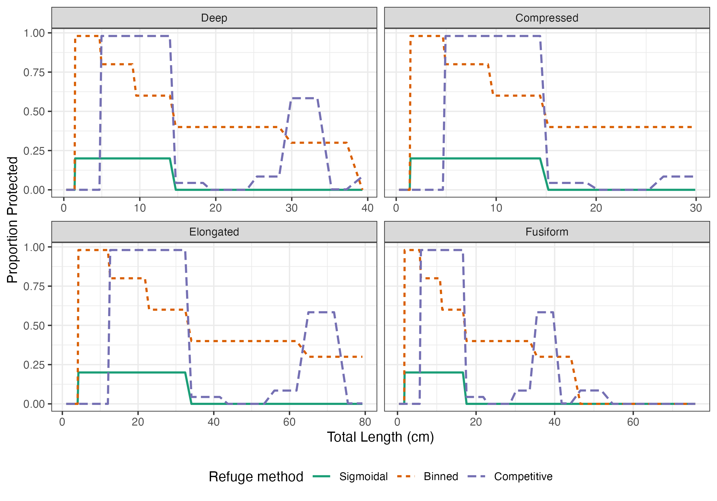
Figure 2. Example refuge profiles for three methods (sigmoidal, binned, competitive) applied to species with different body shapes (deep, compressed, elongate, fusiform).

The package includes several example refuge profiles for tuning and demonstration.

mizerReef’s example models use competitive refuge profiles based on field data. Use the code below to view the built-in Karpata Reef refuge profile:

data(karpata_refuge)
karpata_refuge

##    start_L end_L refuge_density
## 1        0     5     7.53333333
## 2        5    10     1.40000000
## 3       10    15     0.70833333
## 4       15    20     0.28333333
## 5       20    25     0.10000000
## 6       25    30     0.05000000
## 7       30    35     0.04166667
## 8       35    40     0.03333333
## 9       40    45     0.03333333
## 10      45    50     0.04166667

See example models for more details on built-in refuge profiles.

Creating your first model

Skip to Tuning the steady state

Once you have your species parameters (with reef-specific columns) and interaction matrix ready, you can create a MizerParams object using the newReefParams() function. This function extends mizer’s newMultispeciesParams() by adding reef-specific arguments, checking user-supplied parameters, and setting sensible defaults for any missing reef-specific values.

💡 Tip: When creating a new mizerReef model with newReefParams(), you can’t use the competitive refuge method when calibrating biomasses because it is density-dependent.

Use a tuning profile instead.

The best practice if you have refuge density data is to first create a model using the binned method that approximates your refuge profile to reach an initial steady state and calibrate biomasses, then switch to the competitive method. The package includes an example refuge profile for tuning (tuning_profile) that can be used for this purpose.

caribbean_10_model <- newReefParams(species_params = caribbean_10_species,
                                    interaction = caribbean_10_interaction,
                                    method = "binned",
                                    method_params = tuning_profile)

After creating your initial params object, you will typically run through a tuning sequence to calibrate biomasses and adjust reproduction, growth, and unstructured resource parameters to match observed data.

Tuning the steady state

Skip to Exploring results

Reaching a steady state that matches observed biomasses and growth rates is nontrivial and often unique for each system. The procedure developed here was suitable for the Karpata reef data but may differ depending on your calibration data. In brief, the tuning procedure is as follows:

Start with plausible species parameters. Create an initial params object with newReefParams() using a binned or sigmoidal refuge profile that mimics your data.
Reduce the density-dependence of reproduction by reducing the reproduction level. Run to a steady using reefSteady(). Check the resource abundance and scale if needed.
Iterate through calibrateReefBiomass(), matchBiomasses(), matchReefGrowth() and reefSteady() to reach a satisfactory steady state.
Change to your desired refuge method (for example, competitive) using setRefuge(), then re-tune the steady state by iterating/repeating step 3.
Tune the reproduction parameters according to the mizer blog recipe to reach the final steady state.

💡 Tip: One of the most useful summary plots for steady state calibration is plotBiomassObservedVsModel(), which shows the total biomass for each species in your model vs. observed values.

💡 Tip: There are many reasonable ways to reach a suitable steady state. This recipe only represents one approach. You may need to adjust the steps or order depending on your system and data.
The tuning approach used for MizerReef is adapted from the 5-step recipe described in the mizer blog.

For more information on tuning MizerReef models, see the MizerReef Steady State recipe.

Exploring results

Skip to Changing the refuge profile

After reaching a steady state, you should explore the results to ensure they make ecological sense and match expectations for your system. MizerReef provides several plotting functions to help you visualize and interpret your model outputs:

Refuge profile at steady state:
Use [plotRefugeProfile()] to see the proportion of individuals protected by refuge across sizes and species.
```
plotRefugeProfile(params)
```
Diet composition:
Use [plotDiet()] to display the proportion of each prey type in the diet of each predator.
```
plotDiet(params)
```
Total biomass for each species: Use [plotBiomass()] on a projected simulation to view biomasses over time.
```
sim <- project(params)
plotBiomass(sim)
```

💡 Tip: plotBiomass() is mizer’s own function.
mizerReef does not override it — instead it registers a getBiomass() method for mizerReef models so that algae and detritus biomass are automatically included alongside species biomass, regardless of the order in which mizer and mizerReef are loaded.

Productivity by species:
Use [plotProductivity()] to view total productivity for each species.
```
plotProductivity(params)
```

For a full list of available summary and diagnostic plots, see MizerReef summary plots and mizer’s plotting results reference page.

Changing the refuge profile

Skip to Running a simulation

Changing the refuge profile allows you to explore how habitat structure affects model dynamics, such as biomass and productivity. This is useful for simulating habitat degradation or restoration scenarios.

Workflow:

Use newRefuge() to change the refuge profile in your model.
Run reefSteady() several times to reach a new steady state.
Compare results (e.g., biomass and productivity) using built-in plotting functions.

# Change to a non-complex (no refuge) profile
non_complex <- newRefuge(caribbean_10_model, new_method = "noncomplex")

# Run to steady state
non_complex <- non_complex |> reefSteady() |> reefSteady() |> reefSteady()

# Compare biomass and productivity between models. Invertebrates aren't
# included in the productivity calculation, so only plot2TotalBiomass()'s
# legend has the complete set of species - keep that one and drop the
# other, rather than collecting both (which would duplicate the legend
# since the two plots' fill scales don't have identical levels).
all_biom11 <- plot2TotalBiomass(non_complex, caribbean_10_model,
                                name1 = "Flat",
                                name2 = "Complex",
                                stack = TRUE) +
    ggplot2::theme_bw() +
    ggplot2::guides(alpha = "none") +
    ggplot2::theme(legend.position = "bottom")

all_prod11 <- plot2Productivity(non_complex, caribbean_10_model,
                                name1 = "Flat",
                                name2 = "Complex",
                                stack = TRUE) +
    ggplot2::theme_bw() +
    ggplot2::guides(alpha = "none") +
    ggplot2::theme(legend.position = "none")

patchwork::wrap_plots(all_biom11, all_prod11)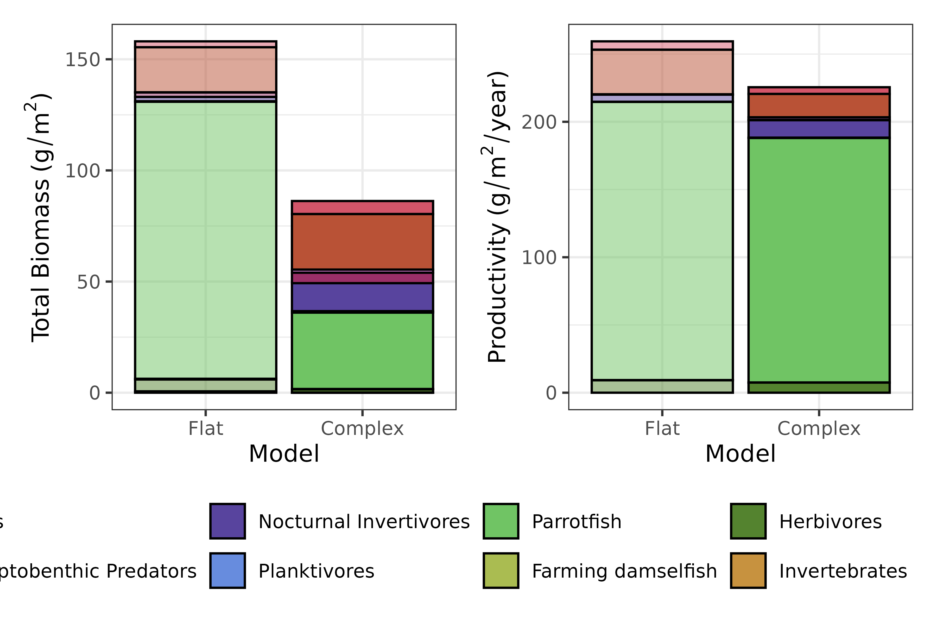

Two-panel plot: left panel shows total biomass for flat vs complex reef, right panel shows productivity for flat vs complex reef. Each panel compares model output for two habitat types.

Figure 3. The biomass (left) and productivity (right) for a model with no predation refuge (non-complex) and a model with predation refuge based on data from Karpata Reef in Bonaire (complex). Colours represent species groups.

As we can see in Figure 3, removing refuge availability reduces total biomass substantially. Total productivity, by contrast, is only modestly affected here – refuge changes which species contribute most to production more than it changes the total. Biomass and productivity can decouple like this because refuge protects juveniles from predation, letting populations skew toward larger, slower-growing individuals: standing biomass goes up, but production per unit biomass goes down.

💡 Tip: If your results look odd after changing the refuge profile, run reefSteady().
It needs to run enough times to reach a new steady state. To learn more about modifying refuge profiles and their parameters, see [setRefuge()].

For more information on the example data used in this vignette, see the mizerReef model description vignette.

Running a simulation

Skip to Links and further reading

Once you have a tuned model at steady state, you can project it forward in time with mizer’s project() function, exactly as you would for a standard mizer model. This section shows two common scenarios: adding fishing pressure, and letting a parameter (here, the refuge profile) change part-way through a simulation.

Simulating fishing pressure

caribbean_10_model already has gear parameters set up, so you can project it forward at a chosen fishing effort. Comparing an unfished run (effort = 0) against a fished run shows the effect of fishing on total biomass:

sim_unfished <- project(caribbean_10_model, effort = 0, t_max = 20,
                        progress_bar = FALSE)
sim_fished <- project(caribbean_10_model, effort = 1, t_max = 20,
                      progress_bar = FALSE)

# Total biomass after 20 years, unfished vs. fished
c(unfished = sum(mizer::getBiomass(sim_unfished)[21, ]),
  fished = sum(mizer::getBiomass(sim_fished)[21, ]))

## unfished   fished 
## 453.4778 276.6875

plotBiomass(sim_fished) +
    ggplot2::theme_bw()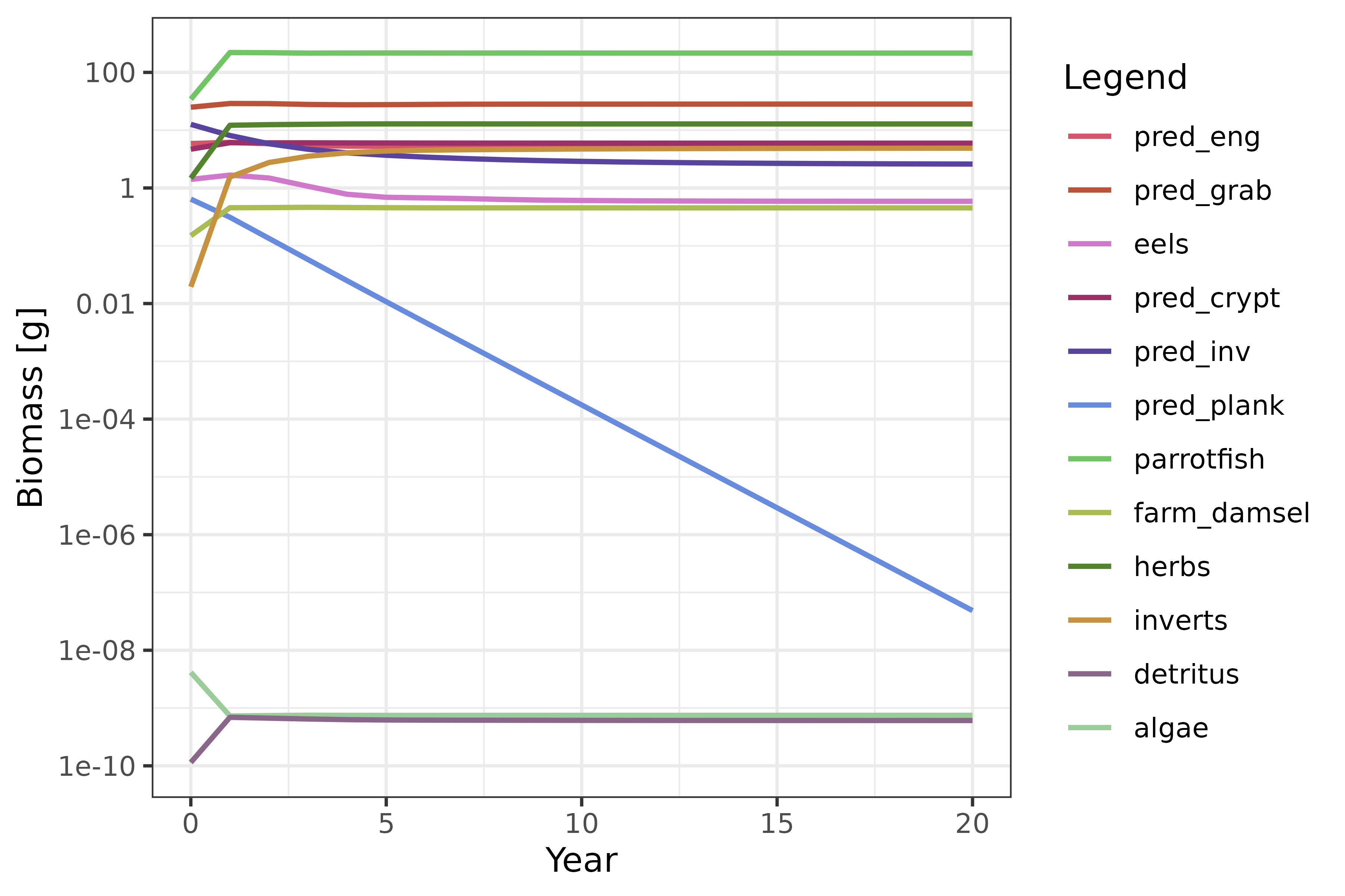

Line plot of total biomass by species over 20 years of simulation with fishing effort 1.

Figure 4. Total biomass over time for the fished simulation.

Yield (the catch taken by the fishery) can be plotted the same way:

plotYield(sim_fished) +
    ggplot2::theme_bw()

Line plot of fishing yield by species over 20 years of simulation with fishing effort 1.

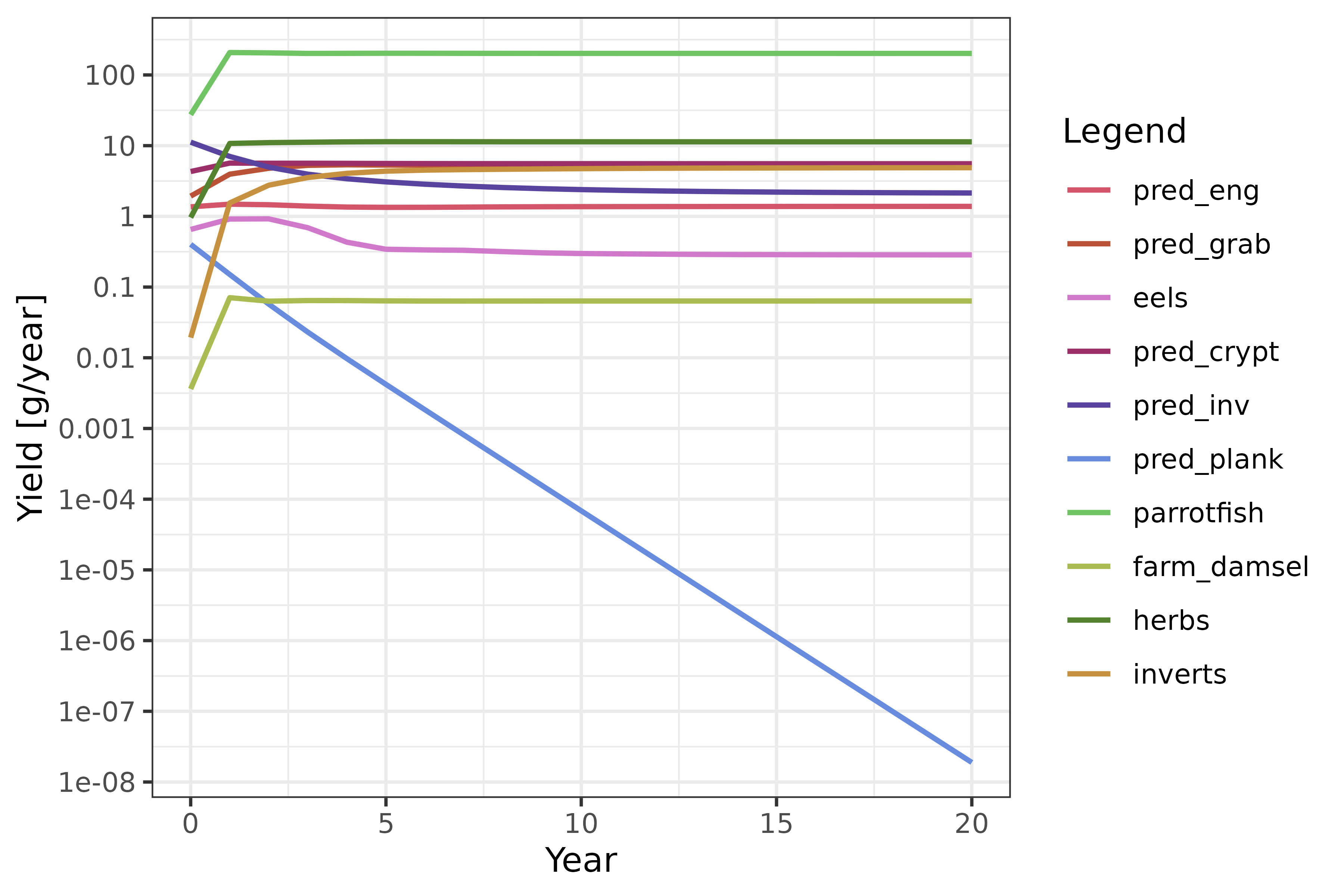
Yield over time for the fished simulation.

See mizer’s own effort and fishing mortality articles for more on setting up gears, selectivity, and effort schedules.

Simulating habitat decline

Refuge parameters can also be changed between projection steps, so a simulation can represent a habitat that is gradually declining (or recovering) rather than staying fixed. The example below uses the sigmoidal method (the simplest of the three refuge methods) purely to illustrate the mechanism: shrink the refuge threshold length and the maximum protected proportion a little each year for five years, projecting one year at a time and carrying the model’s state forward with mizer::finalParams(). The refuge is then left at its final, most-degraded setting for ten more years so the community has time to settle into a new steady state.

params <- newRefuge(caribbean_10_model, new_method = "sigmoidal",
                    new_method_params = list(L_refuge = 10, prop_protect = 0.8))
sim <- project(params, t_max = 1, progress_bar = FALSE)
params <- mizer::finalParams(sim)
params_yr1 <- params

# Refuge threshold length and maximum protection shrinking over 5 years,
# then held fixed for 10 more years to let the community re-equilibrate
L_seq <- c(10, 8, 6, 4, 2)
prop_seq <- c(0.8, 0.6, 0.4, 0.2, 0.05)
n_years <- length(L_seq) + 10

biomass_trend <- numeric(n_years)
productivity_trend <- numeric(n_years)
biomass_trend[1] <- sum(mizer::getBiomass(params_yr1))
productivity_trend[1] <- sum(getProductivity(params_yr1))

for (i in 2:n_years) {
    if (i <= length(L_seq)) {
        params <- newRefuge(params, new_method = "sigmoidal",
                            new_L_refuge = L_seq[i], new_prop_protect = prop_seq[i])
    }
    sim <- project(params, t_max = 1, progress_bar = FALSE)
    params <- mizer::finalParams(sim)
    biomass_trend[i] <- sum(mizer::getBiomass(sim)[dim(sim@n)[1], ])
    productivity_trend[i] <- sum(getProductivity(params))
}
params_yr15 <- params

# Normalise to year 1 so biomass and productivity (different units) can
# share one y-axis and be compared directly on the same plot.
trend_data <- data.frame(
    year = rep(seq_len(n_years), 2),
    pct = c(biomass_trend / biomass_trend[1] * 100,
           productivity_trend / productivity_trend[1] * 100),
    metric = rep(c("Biomass", "Productivity"), each = n_years)
)

ggplot2::ggplot(trend_data, ggplot2::aes(x = year, y = pct, color = metric,
                                         shape = metric, linetype = metric)) +
    ggplot2::geom_line() +
    ggplot2::geom_point(size = 2) +
    ggplot2::scale_color_manual(values = c(Biomass = "#1B9E77", Productivity = "#D95F02")) +
    ggplot2::labs(x = "Year", y = "% of year-1 value", color = NULL, shape = NULL, linetype = NULL) +
    ggplot2::theme_bw()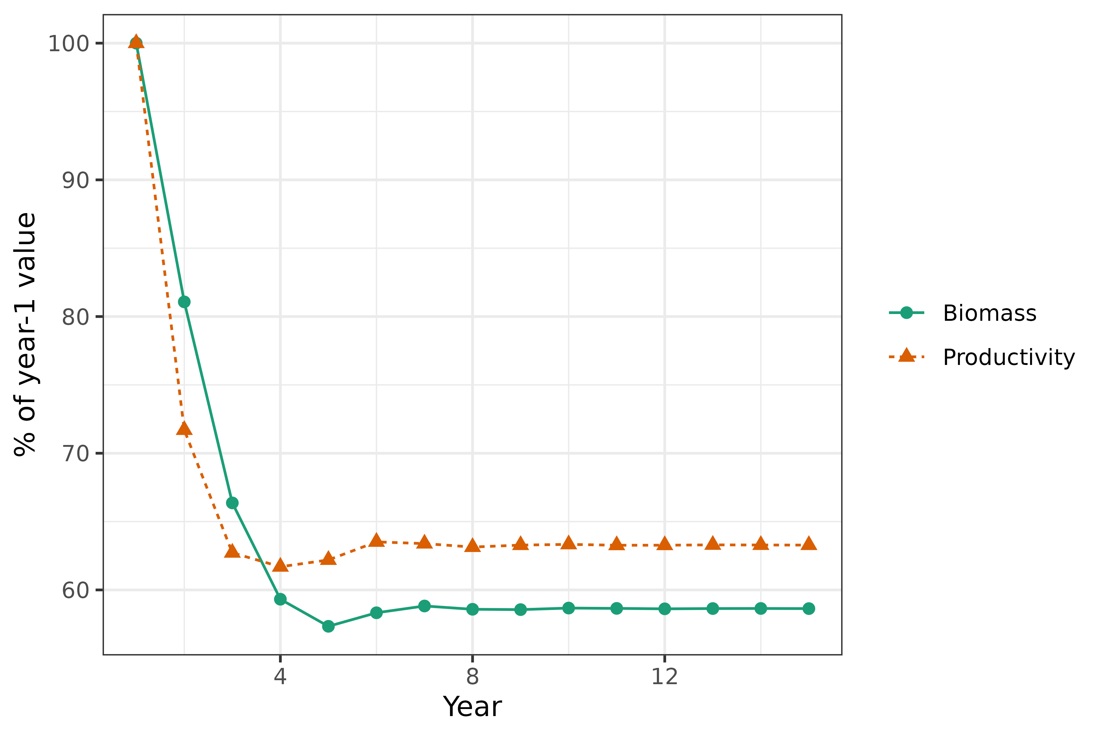

Line plot of total biomass and productivity over fifteen years as the refuge threshold length and maximum protected proportion shrink then hold, ending at different levels relative to their starting values.

Total biomass and productivity over fifteen years as refuge shrinks then holds at its final degraded state, each shown as a percentage of its year-1 value so the two can share one axis.

Biomass ends up lower than where it started (about 90% of its year-1 value), but productivity actually settles at a higher new steady state (about 125%). Aggregate totals like these can hide a lot of detail, though - looking at individual species groups tells a very different story:

species_names <- species_params(caribbean_10_model)$species
species_comparison <- data.frame(
    species = rep(species_names, 2),
    year = rep(c("Year 1", "Year 15"), each = length(species_names)),
    biomass = c(as.numeric(mizer::getBiomass(params_yr1)),
               as.numeric(mizer::getBiomass(params_yr15)))
)

ggplot2::ggplot(species_comparison, ggplot2::aes(x = species, y = biomass, fill = year)) +
    ggplot2::geom_col(position = "dodge") +
    ggplot2::scale_y_log10(limits = c(1e-3, NA), oob = scales::squish) +
    ggplot2::labs(x = "Species Group", y = expression("Biomass (g/m"^2*", log scale)"), fill = NULL) +
    ggplot2::theme_bw() +
    ggplot2::theme(axis.text.x = ggplot2::element_text(angle = 45, hjust = 1))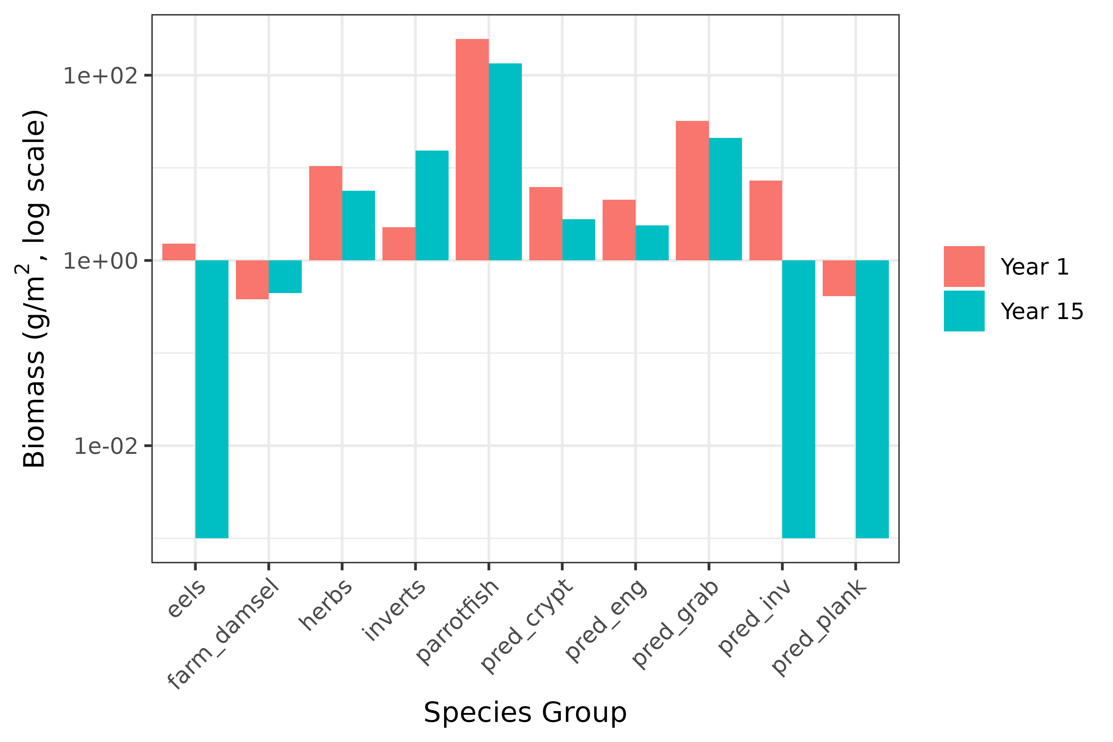

Grouped bar chart of biomass by species group, comparing year 1 and year 15, on a log scale. Several bars for year 15 are clipped at the floor of the axis, indicating functional extinction.

Species-level biomass before (year 1) and after (year 15) refuge loss, log scale. Several groups collapse to near zero.

Four of the ten species groups - Engulfers, Eels, Nocturnal Invertivores and Planktivores, all species that rely on refuge for protection - collapse to functionally zero biomass. Parrotfish (the dominant group by biomass) barely changes, and Invertebrates increase substantially, which is why the aggregate biomass and productivity trends above look like a moderate decline rather than a multi-species collapse. plotRelativeContribution() makes the same point from a different angle, comparing how much each species group contributes to abundance, biomass, and productivity before and after:

patchwork::wrap_plots(
    plotRelativeContribution(params_yr1) + ggplot2::ggtitle("Year 1 (with refuge)") + ggplot2::theme_bw(),
    plotRelativeContribution(params_yr15) + ggplot2::ggtitle("Year 15 (refuge lost)") + ggplot2::theme_bw()
) +
  patchwork::plot_layout(guides = "collect") &
  ggplot2::theme(
    legend.position = "bottom",
    legend.title = ggplot2::element_blank(),
    legend.text = ggplot2::element_text(size = 8),
    legend.key.height = grid::unit(0.35, "cm"),
    legend.key.width = grid::unit(0.6, "cm"),
    legend.spacing.x = grid::unit(0.1, "cm")
  )

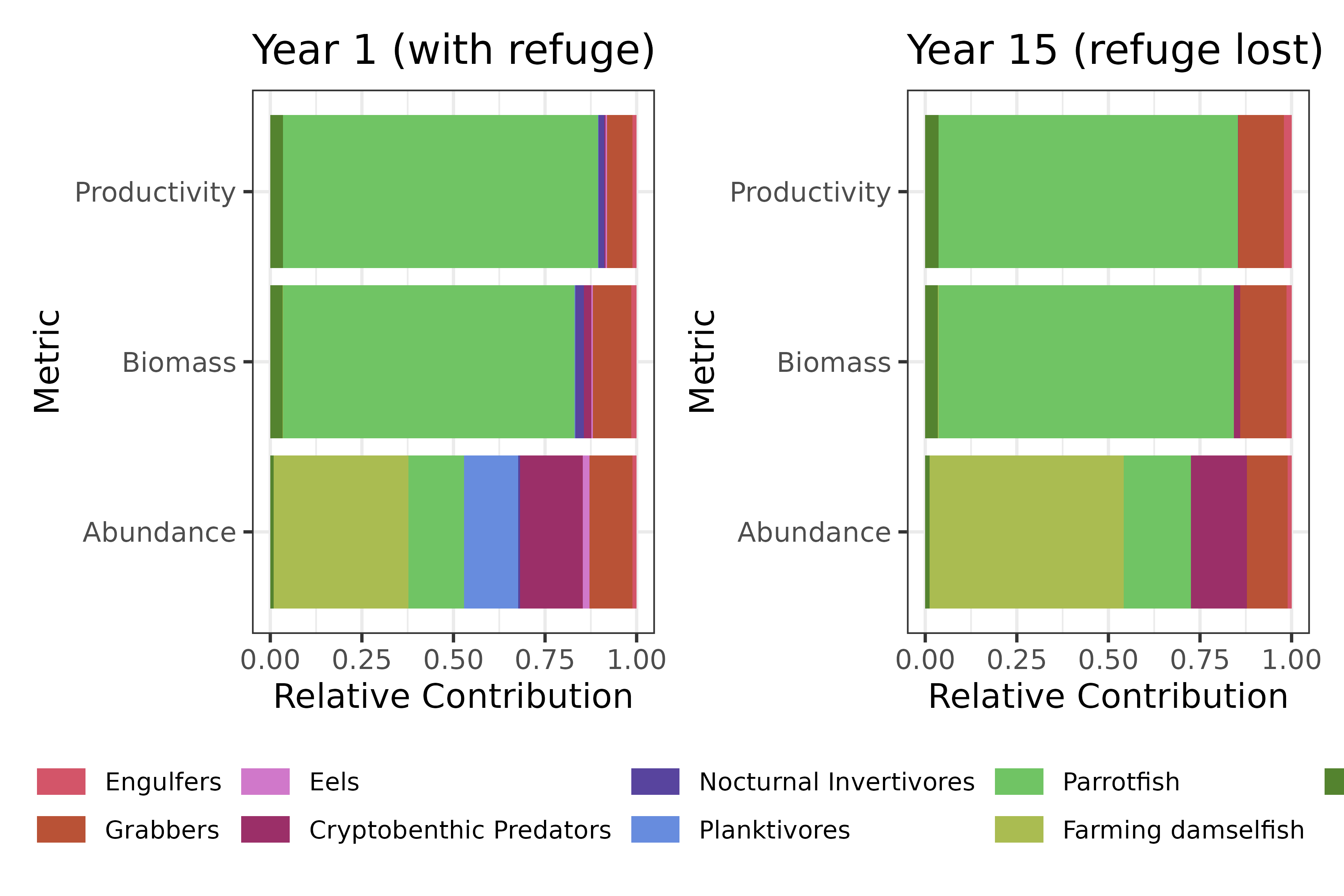
Two side-by-side stacked bar charts comparing the relative contribution of each species group to abundance, biomass and productivity, one for year 1 and one for year 15. The abundance panel shows the Planktivores' share present in year 1 has vanished by year 15.

Relative contribution of each species group to abundance, biomass, and productivity, comparing year 1 (with refuge) and year 15 (refuge lost).

The Planktivores’ share of total abundance in year 1 (the blue band) is entirely gone by year 15 - direct visual confirmation of the collapse shown in the previous figure, this time in terms of each group’s relative share rather than its absolute biomass.

💡 Tip: This is a mechanism demo, not a calibrated analysis.
Switching refuge methods abruptly (as done here) skips the tuning workflow described in Tuning the steady state; for a real analysis, follow that recipe after switching methods, not just after creating the model. MizerReef also supports fully specified, data-driven habitat-degradation trajectories via [setDegradation()] and [reefDegrade()] for the "competitive" refuge method — see their reference pages for details.

Links and further reading

Skip to Model description context

MizerReef documentation and tutorials:

MizerReef documentation: Main package documentation and reference manual
MizerReef model description vignette: Detailed explanation of model structure and example workflows
MizerReef Steady State recipe: Step-by-step guide for tuning models to steady state
Example models and built-in data: Reference for example species, interaction matrices, and refuge profiles

Plotting and function references:

MizerReef summary plots: List of available summary and diagnostic plots
setRefuge() function documentation: Details on modifying refuge profiles and parameters
Mizer plotting results reference: Reference for plotting functions in mizer

General mizer resources:

Official mizer getting started guide: General introduction to mizer

Further research:

Modelling Coral Reef Futures: Exploring the role of structural complexity in sustaining ecosystem services (PhD Thesis, VUW): In-depth research and context for MizerReef

Session info

## R version 4.6.1 (2026-06-24)
## Platform: x86_64-pc-linux-gnu
## Running under: Ubuntu 24.04.4 LTS
## 
## Matrix products: default
## BLAS:   /usr/lib/x86_64-linux-gnu/openblas-pthread/libblas.so.3 
## LAPACK: /usr/lib/x86_64-linux-gnu/openblas-pthread/libopenblasp-r0.3.26.so;  LAPACK version 3.12.0
## 
## locale:
##  [1] LC_CTYPE=C.UTF-8       LC_NUMERIC=C           LC_TIME=C.UTF-8       
##  [4] LC_COLLATE=C.UTF-8     LC_MONETARY=C.UTF-8    LC_MESSAGES=C.UTF-8   
##  [7] LC_PAPER=C.UTF-8       LC_NAME=C              LC_ADDRESS=C          
## [10] LC_TELEPHONE=C         LC_MEASUREMENT=C.UTF-8 LC_IDENTIFICATION=C   
## 
## time zone: UTC
## tzcode source: system (glibc)
## 
## attached base packages:
## [1] stats     graphics  grDevices utils     datasets  methods   base     
## 
## other attached packages:
## [1] knitr_1.51              mizerReef_2.0.1         mizerExperimental_3.2.0
## [4] mizer_3.2.1            
## 
## loaded via a namespace (and not attached):
##  [1] plotly_4.12.1      sass_0.4.10        generics_0.1.4     tidyr_1.3.2       
##  [5] stringi_1.8.9      digest_0.6.39      magrittr_2.0.5     timechange_0.4.0  
##  [9] evaluate_1.0.5     grid_4.6.1         RColorBrewer_1.1-3 fastmap_1.2.0     
## [13] plyr_1.8.9         jsonlite_2.0.0     httr_1.4.8         purrr_1.2.2       
## [17] viridisLite_0.4.3  scales_1.4.0       textshaping_1.0.5  jquerylib_0.1.4   
## [21] cli_3.6.6          rlang_1.3.0        withr_3.0.3        cachem_1.1.0      
## [25] yaml_2.3.12        otel_0.2.0         tools_4.6.1        reshape2_1.4.5    
## [29] dplyr_1.2.1        ggplot2_4.0.3      assertthat_0.2.1   vctrs_0.7.3       
## [33] R6_2.6.1           lubridate_1.9.5    lifecycle_1.0.5    stringr_1.6.0     
## [37] fs_2.1.0           htmlwidgets_1.6.4  ragg_1.5.2         pkgconfig_2.0.3   
## [41] desc_1.4.3         pkgdown_2.2.1      pillar_1.11.1      bslib_0.12.0      
## [45] gtable_0.3.6       glue_1.8.1         data.table_1.18.4  Rcpp_1.1.2        
## [49] systemfonts_1.3.2  xfun_0.60          tibble_3.3.1       tidyselect_1.2.1  
## [53] farver_2.1.2       patchwork_1.3.2    htmltools_0.5.9    labeling_0.4.3    
## [57] rmarkdown_2.31     compiler_4.6.1     S7_0.2.2           splus2R_1.3-5